Methodology

PROJECT HOME | BACKGROUND | METHODOLOGY | RESULTS AND DATA | REFERENCES

The primary goal of this project was to develop and document methods for quantifying land use change using remotely sensed imagery and other freely available data sources. The following section is an overview of the process that we used to determine land use change, from acquiring the original images to the change detection methodology. If you are interested in more specific process documentation, with step-by-step procedures, please contact us.

First, click on the graphic below for a generalized flow chart of the process.

1 Data Acquisition

2 Image Pre-Processing

3 Image Classification

4 Land Use Determination

1 Data Acquisition

1a Landsat Images

The moderate resolution of Landsat was ideal for this project given the large landscape involved and the three time-step periods. The time-steps were determined to take advantage of the most recent images available from the PNW office (2004) and the first thematic mapper (TM) images available in 1988; 1996 is the eight-year mid-point between the two dates. All of the 2004 images were precision geocorrected at the 1G level, most of the 1996 images were terrain corrected (processing level 10), and most of the 1988 images were geometrically corrected. The 24 images (8 for each year) were close in time during the summer to avoid seasonal and phenological differences in vegetation types and other seasonal land cover differences (Howarth and Boasson 1983, Song and Woodcock 2003). Each image was imported into the IMAGINE (.img) file type, from the USGS NLAPS form or.tiff, for further processing The specific images acquired for this project are listed below.

Table 1. Landsat Images

1b Ancillary Data

Ancillary data (listed in Table 2) was collected to determine the analysis area (non-federal lands in western Washington) and to aid in the segmentation of the coarse scale classifications (floodplain and elevation data).

Table 2. Ancillary Data

2 Image Pre-Processing

As discussed earlier, all of the images used in this project were processed to some degree either by the USGS or the USFS (see Table 3 for a description of the processing for each level of geocorrection). In an attempt to save time and resources, it was decided that the image processing done ahead of time was sufficient for this project.

Table 3. USGS Geometric Corrections

While the atmosphere causes increases in the estimates of low reflectance and decreases the highly reflective surface estimate, this project did not correct for atmospheric distortion. Pax-Lenney et al. (2001) showed that correction for atmospheric interference did not statistically improve image classification, and Song et al. (2001) found that as long as the training data was from the same image that was to be classified, and multiple images were classified separately, atmospheric correction was unnecessary. Since this project aimed to provide easily repeatable and time-efficient results, this step was determined unnecessary; additionally, as discussed later, all training samples were taken from individual images. Finally, the change detection that was done in the land use change step was done with classified polygon layers, rather than comparing spectral values.

Although the 2004 images were precision geocorrected, a small amount of additional geometric transformation was necessary to align the images perfectly; 2004 was chosen as the base year for all other images to be registered to.

2b Image Registration

Image registration is often very time-consuming, sometimes taking months to collect an adequate number of ground control points (GCPs). In order to produce accurately registered images in a relatively short amount of time, this project took advantage of a free application called ITPFIND that automatically finds image reference points for image rectification. It was written by Robert Kennedy from the USDA Forest Service, Pacific Northwest Research Station at Oregon State University. ITPFIND was written to run in IDL ®, a software program for "data analysis, visualization, and cross-platform application development."

ITPFIND creates input and reference X and Y point text files for import to ERDAS IMAGINE ® or other image rectification software; the application and documentation area available as a free download (http://www.fsl.orst.edu/%7Ekennedyr/ ) and Phil Hurvitz, at the University of Washington, wrote detailed instructions specifically for this project ( http://gis.washington.edu/phurvitz/itpfind/ ).

2c Analysis Area

Clipping the images to the areas of interest significantly reduces processing time for each image. Areas off the coast of Washington and within large Forest Service and National Park lands were removed from the images by using the Subset Image command in ERDAS Imagine.

The first step was to create clipping shapefiles for use with an ArcView 3.x clipping script. The script uses a single clipping shapefile of Western Washington and then for each image creates a unique clipping shapefile. The process steps below have been generalized for reporting purposes but should be easy to follow for an experienced GIS analyst. The data sources listed in Table 2 were used to create the clipping shapefile.

Gifford Pinchot National Forest, Olympic National Forest, Mount Baker/Snoqualmie National Forest and National Park Service lands were merged into a federal land feature class. Other public entities like the Bureau of Land Management, the Fish and Wildlife Service and the Washington State Department of Natural Resources were not excluded from the analysis as their exclusion would not have significantly affected processing time.

A western Washington shapefile was generated by selecting only those counties west of the Cascade crest and merging them into a single shape. This shapefile, and the federal lands shapefile, were simplified using a 30-meter filter to speed processing time for the subsequent steps since retaining such accurate boundaries is of no use after being buffered. This simplified western Washington shapefile was buffered by 5000 meters to create an external shapefile, and the simplified Federal Land shapefile was buffered by 1000 meters to create an internal shapefile.

Small islands and slivers (less than 10 square kilometers) were removed in both the external and internal shapefiles. The area included in the internal shapefile was erased from the external shapefile, and the result was clipped along the Cascade crest to create a western Washington analysis area shapefile.

2d Image Clipping

The second step was to generate the individual image clipping shapefiles using a script in ArcView. The script gets the extent of each image and then extracts a new shapefile for that image from the master clipping shapefile (western Washington analysis area). These shapefiles were used in ERDAS Imagine to generate areas of interests (AOIs) to subset the images.

The third step was to clip the referenced images with the newly created clip shapefiles. This was done in ERDAS Imagine, using the defined AOIs and the Subset Image tool. A batch method was used to allow for the processing to occur at night when the computers were not in use. Using the batch method resulted in each image taking about 2 minutes to setup for batch processing and then 10 minutes to process.

3 Image Classification

3a Image Classification

Two segmentation levels were used to differentiate between large areas of relatively homogeneous land cover and small areas of development (see Classification Schematic below). This resulted in two different land cover classifications: a general land cover classification (i.e. forest or irrigated lands) and a developed (i.e. concrete, rooftops) land cover classification.

Young forest and irrigated grass land cover classes are difficult to differentiate in landsat imagery. To assist in the differentiation of light green forest and irrigated agricultural lands a floodplain layer was used to segment the imagery for the coarse land cover classification. In addition, elevation classes were used to help differentiate between cleared forestland and bare agricultural soils. The eCognition classification rules were constructed to assign higher probabilities to classes based on the objects location inside or outside of a floodplain and higher or lower in elevation. Using the floodplain and elevation layers increased classification accuracy by helping to differentiate between spectrally similar objects with different land uses.

The following table describes both the coarse and fine classifications.

Table 4. Land Cover Classifications

The following land cover classifications were grouped into larger classes (groups, shown in bold font) in order to calculate contiguous land cover characteristics.

•  Dark Forest, Light Forest and Regeneration land cover classes: Forest

•  Irrigated, Soil and Mixed/Ag Soil land cover classes: Agriculture

•  Residential and Urban land cover classes: Developed

•  Cloud land cover class: Clouds

•  Shadow land cover class: Shadow

•  Unclassified land cover class: Unclassified

The built-up land cover classification was not grouped into the land cover groups; rather, it was used to calculate percent developed and development density within the larger land cover groups.

•  Built-up:Percent developed and development density

The figure below shows the flow from the original Landsat image, classified at both the fine- and coarse-scales, to determination of land use (which is discussed in section 4, Land Use Determination, below).

Classification Schematic

3b Re-clipping No Data Areas

When eCognition exports the classified.img file, it does not differentiate between "NoData" pixels and "unclassified" pixels. Our classifications include both NoData pixels and actual unclassified pixels, and we need to differentiate between the two. Our original clipping shapefiles were created by the intersection of the "analysis area" polygon and the rectangular extent of the original images, therefore clipping by the original clipper shapefiles does not eliminate NoData areas from the classified rasters. Thus, we reclassified the actual NoData values, while keeping the correct classification for actual unclassified objects, using a series of python scripts.

3c Agreement Matrix

In order to assess the accuracy of the initial classification results, a simple correlation matrix was run to compare the overlapping areas of the images. Using a series of python scripts and Excel spreadsheets, agreement matrices were calculated. The correlation between the overlapping, classified images are shown in Table 5.

Table 5. Classified Image Correlation

3d Mosaic

Using the original registered Landsat images, the images were hierarchically arranged in the table of contents in an ArcMap document to create the least area of cloud, haze, and glare. During a mosaic process, however, a user will often want just a portion of an image rather than putting one entire image at the top (or bottom) of the hierarchy. Therefore, in order to achieve the best mosaiced image, some of the images had to be clipped before being added to the mosaic order.

If an image needed to be clipped to include just a portion of the area (for example, one image is completely cloud free except for a small area in one corner), a new polygon feature class with the same spatial properties of the respective image was created in ArcCatalog. This blank feature class was added to the ArcMap document and was edited, using the sketch tool, to cover the portion of the image that is best used in the mosaic process. The figure below shows the clipper (in purple) as to avoid the clouds on the left-hand side (within the white circle). The neighboring image contained much cloud cover, but was clear where this image was cloudy. Before clipping the image with this new feature class, it was necessary to perform a visual check to make sure that the image below (or above) would still result in a complete mosaic. Lastly, since the raster calculator cannot clip more than 3 bands, it was necessary to use ERDAS Imagine's data prep/subset image tool.

Clipper to avoid clouds

4 Land Use Determination

As discussed earlier, land cover is the biophysical characteristics of the landscape, while land use is made up multiple land cover types. Determining land use from satellite images require a series of overlay processes that neither eCognition, ArcGIS, or ArcSDE could handle due to large file sizes or massive computer RAM requirements. Additionally, it was necessary to devise a method that could be easily run again, with new input data, and altered to reflect different land use characteristics and definitions. A series of AMLs, written to run in ArcInfo Workstation, are described below. For more information about the AMLs, please contact us.

Create Land Use Polygons (CREATELCPOLYS.aml): Image objects from eCognition were converted to ArcInfo polygon coverages and then joined with the eCognition image object attributes. To help with land use classification, land covers were organized into classes and grouped into like types (i.e. forest, mixed, built).

Set the Minimum Mapping Unit (ELIMINATELC.aml): In order to reduce the amount of data in each GRID, small polygons were eliminated (land uses are usually large in size, unlike land cover, so it was assumed that data quality would not be compromised). Using Arc and ArcPlot, any polygons less than 10-acres and not identified as water by the WADNR were eliminated. This resulted in "land use polygons" - which formed the spatial arrangement for the remaining attribute analysis.

Add the Land Use Field (ADDLUFIELDS.aml): The additional attribute fields needed to arrive at land use were added to the land cover attribute table using ARC.

Calculate Contiguous Acres (CALCONTIGACRES.aml): Some of the land use definitions required a calculation of contiguous acres of similar land covers. Adjacent land cover classifications were combined to create contiguous areas of land cover classes. Contiguous land cover classification acres were calculated as a metric for calculating land use. Additionally, adjacent land cover classification groups were combined to create contiguous areas of similar land cover classes. Contiguous land cover group acres were calculated as a metric for calculating land use.

Calculate Development Statistics (DEVSTATS.aml): In addition to contiguous acres, the land use definitions included development statistics: number of acres of each polygon that are developed, percentage developed, number of cells developed, number of development clusters, density of clusters per square mile, and more. Unioning land use cover with built-up cover (from the fine-scale built-up layer), by connecting to an Access database, exporting the attribute tables, and running a selection query using an AML, creates these development statistics. The percent developed is the amount of concrete or other developed land cover that is within each land use polygon. The percentage developed of each land use polygon was calculated by overlaying the fine scale developed land cover classification on the dissolved coarse scale general land cover classification. Development density is the number of individual developments per square mile. The fine scale developed land cover classification was grouped into individual developments. Developments could be of any size ranging from approximately ¼ acre to 169,000 acres in the Seattle metropolitan area. The number of these unique developments in each land use polygon was normalized to a per square mile development density figure.

Determine Land Use (LANDUSE.aml): Calculating land use involved running an AML to put each polygon is one of the groups listed in the first column in Table 6, based on the corresponding requirements listed in the subsequent columns. The land use polygon coverage developed with the previous AMLs are necessary for the calculation of land use. Each land use polygon was coded with a number in ascending order: the most wild land use (wildland forest) has the lowest number and the most developed land use (urban) has the highest number. The land uses determined in this analysis are described in Table 6 and described in much more detail below the table.

Table 6. Rules Used to Calculate Land Use

•  Wildland Forest

•  Description: Industrial and non-industrial forestlands, parks, municipal watersheds and other forested lands that have very few paved roads or residential developments.

•  Definition: At least 640 contiguous forest group acres and no more than 5% developed with a development density of 4 per square mile or less. The land use polygon must be in a forest land cover classification group.

•  Rural Forest

•  Description: A mix of forestland types with some dispersed residences.

•  Definition: At least 640 contiguous forest group acres and no more than 20% developed with a development density of between 4 and 8 per square mile. Contiguous forest group acres less than 640 and no developments or the land use polygon is greater than 640 acres and no more than 5% developed. The land use polygon must be in a forest land cover classification group.

•  Other Forest :

•  Description: Areas that are primarily forest but have too many developments to be considered rural forest.

•  Definition: Any remaining land use polygons that are in a forest land cover classification group and not wildland forest or rural forest.

•  Intensive Agriculture:

•  Description: Agricultural and livestock lands dominated by irrigated crops or grassland, bare soil and dispersed farm buildings.

•  Definition: At least 640 contiguous irrigated or soil acres and no more than 5% developed with a development density of 9 per square mile or less. Contiguous irrigated or soil class acres less than 640 and less than 1% developed or mixed ag/soil land cover classification and less than 1% developed.

•  Mixed Agriculture:

•  Description: A mix of agricultural and livestock lands with some additional residences unrelated to agriculture and an occasional small development. Often includes non-irrigated and cleared lands and occasional industrial buildings.

•  Definition: At least 640 contiguous class acres in an agricultural land cover group and no more than 20% developed with a development density of 12 per square mile or less.

•  Other Agriculture:

•  Description: Agricultural and cleared lands that have a development density equated to 20 or 40 acre parcels that may be single-family residences, hobby farms or small agricultural operations.

•  Definition: Any remaining land use polygons that are in an agriculture land cover classification group and not intensive agriculture or mixed agriculture.

•  Low-Density Residential:

•  Description: Large areas of development in suburban and rural settings where parcel sizes are large and the landscape is dominated by roads, homes and commercial buildings.

•  Definition: At least 40 contiguous class acres that are in a forest or agricultural land cover classification group and are between 20% and 50% developed.

•  High-Density Residential:

•  Description: Large areas of development in dense urban settings or in large rural developments. Small parcel sizes. Around 50% of the land surface is impervious surface like roads, roofs, sidewalks and driveways.

•  Definition: Land use polygons that are in the developed land cover classification group and less than 50% developed or less than 40 contiguous class acres and greater than 50% developed or in a non-developed land cover classification group and greater than 50% developed.

•  Urban:

•  Description: Dense urban development. Over 50% of the land surface is impervious surface with little vegetation. Airports, industrial parks, urban centers, multi-family residential and very high density residential development.

•  Definition: At least 40 contiguous class acres that are in a developed land cover classification group and greater than 50% developed.

•  Water:

•  Description: Oceans, lakes, reservoirs and streams.

•  Definition: Any land use polygon in a water land cover classification group.

•  Unknown:

•  Description: Any land cover that could not be classified due to spectral ambiguity, cloud cover, haze or shadow.

•  Definition: Any land use polygon in an unknown land cover classification group.

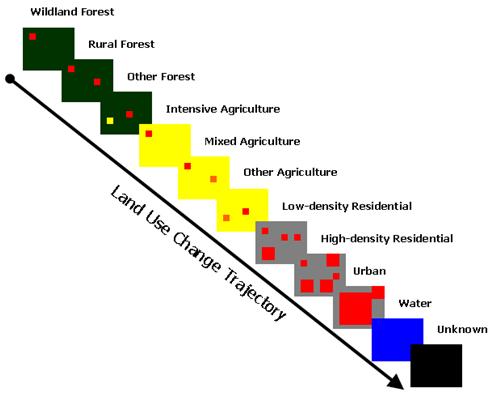
Calculating Land Use Change (CHANGE.aml): The final step in the project is the calculate change from one land use type to another. Each years polygon land use coverage was converted to GRID for analysis of change. Using the combine function in GRID, the change matrix is calculated. As can be expected with multiple land use classes, the number of possible changes (forest to urban, forest to agriculture, agriculture to forest, etc.) could be quite large. For simplicity, a one-way trajectory (shown in the figure below) for change was assumed: a land use can only become more developed, not less developed. This methodology was chosen to minimize the effects of misclassification in intermediate years but has the side-effect of likely overstating land use change since land can not progress to a less developed state and since any misclassifications will be assumed to be the more developed.

Change Trajectory

Land Use Accuracy

An accuracy assessment of the final land use classifications, using high-resolution aerial photography for 94 stratified random points through western Washington, resulted in an overall accuracy of 84% (Table 7). This result is consistent with many other land cover and land use classifications. The largest sources of error were distinguishing between transitional and rural, mixed agricultural lands common in areas undergoing scattered conversion of forest land to rural hobby farms and pastures.

Table 7: Land use classification accuracy matrix

Continue to Results and Data