Lesson 9: Introduction to the
Landscape Management System (LMS)

Review and Introduction

In earlier lessons, you learned how to establish and take measurements in sample inventory plots. In Lesson 8, you used a tool called the Inventory Wizard to enter your inventory (stand and tree) data into your computer and generate a portfolio for use with the Landscape Management System (LMS). Now it is time to start using LMS and putting your inventory data to work!

This lesson is not intended as a comprehensive instruction manual for LMS. Rather, it is to familiarize you with some of the most frequently used features of the program. You have a full-featured version of LMS so you can go beyond these basics and explore on your own.

Learning Objectives:

By the end of this lesson, you will be able to use LMS to:

1. Generate basic forestry tables
2. Generate stand images
3. Simulate growth of forest stands into the future
4. Simulate thinning, harvesting, and planting  and see how these scenarios impact future stand conditions
5. Find more comprehensive resources on the use of LMS

Materials Needed:

1. Windows®-based computer
2. Microsoft ® Excel¹ (recommended)
3. LMS version 2.x software²
   
   

I. Exploring LMS tables

Some of the most important outputs in LMS are the tables. The numbers in the tables can tell us a lot about the stands they represent. LMS has many tables; we will look at three that are particularly useful for describing the forest.

Open your portfolio as you did at the end of Lesson 8. Once it is open, go to Analysis: Tables to bring up the Select Table window (Figure 9-1).  You will see several options here. From the list of tables, select the Summary table. Under Analyze using, make sure that standing trees, all years, and all stands are selected (default values). Under Output, select Spreadsheet to have LMS open the table as a Microsoft® Excel spreadsheet (recommended). If you do not have Excel on your computer, you can also select the Text Editor option to generate the table as a text file.³ After selecting these options, click OK and the Summary table will be generated.

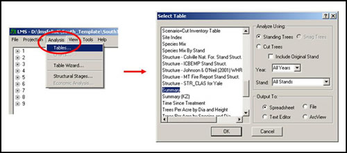Figure 9-1: Generating a table in LMS.

The summary table has quantitative information about the trees in each stand, giving summary statistics by species and total.  There are a number of figures in this table; here are a few of the key ones:

• TPA: Trees per acre – This is one of the most basic statistics used when describing a stand – expressing the density of the stand as the number of trees on a per acre basis. TPA can also give you a sense of average spacing:
  
  
  • 435 TPA = 10-foot spacing
  • 300 TPA = 12-foot spacing
  • 195 TPA = 15-foot spacing
  • 110 TPA = 20-foot spacing
  • 50 TPA = 30-foot spacing

   

• TBA: Total basal area per acre – Basal area is the cross sectional area a tree trunk at breast height. Total basal area per acre is the sum of the basal area for all the trees in the stand on a per acre basis. Because total basal area is a function of both the number and size of trees, it can be used as an indicator of whether or not a stand should be thinned.
  
  
• AveDBH: Average diameter – This is a simple average of the diameter at breast height value for all the trees in the stand (i.e. the sum of all diameters divided by the number of trees).

• DBHq: Quadratic mean diameter (QMD) – This is slightly different from average diameter. In this case, the average basal area is computed, and then the average basal area value is converted to the corresponding diameter. By doing it this way, the average diameter will be weighted toward the larger, overstory trees (which are usually of more interest from a management perspective). If the quadratic mean diameter is significantly different from the average diameter, it is an indication that there are many very small trees mixed with a few larger ones.

• AveHt: Average height – A simple average of all the tree heights in the stand (i.e. the sum of all heights divided by the number of trees).
  
  
• TBFVolPerAcre: Total board-foot volume per acre – This is an estimate of the total volume of wood per acre in the stand, expressed in board feet using the Scribner scale, which is a commonly used measure when selling timber. There are additional columns expressing volume in cubic feet and merchantable cubic feet.

The important forest statistics described above usually involve laborious hand calculations, but they can be computed quickly with a program like LMS. The numbers in this table tell you a lot about the stands. Start thinking about what can discern from this table. What species are present in each stand? How dense are your stands? How uniform are your stands?

When looking at the summary table, it can be helpful to look at one species at a time. On the Excel menu bar, there should be a new option called LMS⁴. Go to LMS: AutoFilter, which will cause small arrows to appear at the top of each column (Figure 9-2).  Now in the species column, click the arrow next to species and select one of the options. This will show statistics only for that species.

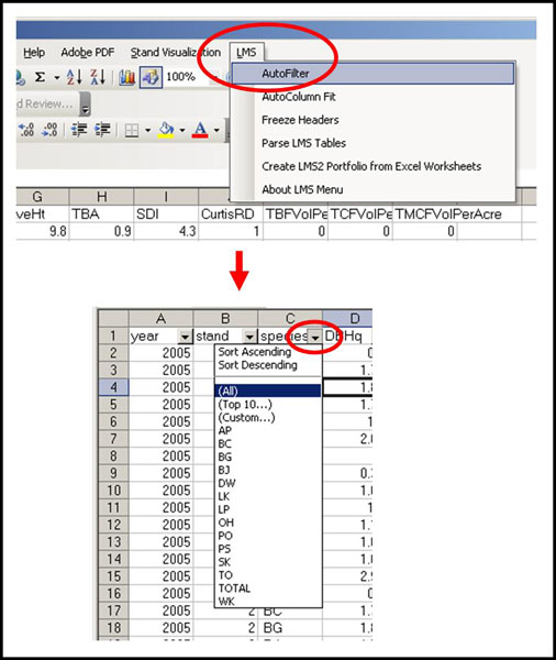Figure 9-2: A new LMS menu item in Excel will allow you to filter your tables.

Close the summary table (after saving the file if you wish) and return to the main LMS window. Click the plus next to one of your stands to reveal the inventory year below (Figure 9-3). Try right-clicking on the year in the main LMS window and select Tables from the drop-down menu.  This is another way to bring up the select table window.  Notice on the right that the stand drop-down box has been set to the stand you chose instead of All Stands and the year has been set to the year you chose instead of All Years.  Select the table called Trees Per Acre by Species and Dia and click OK.  Notice how only the one stand is included this time. This table shows the number of trees per acre in the stand by diameter class (e.g. 0-2”, 2-4”, etc.). If you are working in Excel or comparable spreadsheet program, you can use spreadsheet program’s chart function to create a chart of this table as another way to analyze the data (Figure 9-4). If you are not familiar with making charts, consult the help file or instruction manual for your spreadsheet program.

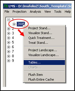Figure 9-3: You can right-click a year under each stand for easy access to tables and other features.

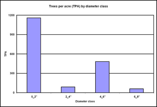Figure 9-4: Once a table is open in Excel, you can use Excel to create useful charts. This chart shows the number of trees per acre by diameter class for a young loblolly pine plantation.

Now try opening a third table: Species Mix by Stand. This table shows the proportion of each species in the stand on a trees per acre basis (proptpa), a basal area basis (propba), and a volume basis (propvol). Try using Excel to create pie charts of these.

Go beyond these instructions and play with other capabilities of LMS.  You will see quickly that LMS is very versatile.

II. Creating stand visualizations

“A picture is worth 1,000 words.” While the numbers from the summary table and other tables are useful, a picture may communicate much better what a stand is like. From the main LMS window, go to View: Stand (Figure 9-5).  Select a stand and a year, and then click OK to bring up the visualization in a separate program window for the Stand Visualization System (SVS) (Figure 9-6).  Go to SVS Options: Screen Layouts (Figure 9-7) and see what some of the different options (0-12) look like.  Note the difference between perspective view, overhead view, and profile view (all three are shown in Figure 9-6).  Also notice some of the different charts available.  Select the perspective view (4) and now go to SVS Options: Perspective view options (Figure 9-8). Move some of the slider bars around and see how that changes the picture.

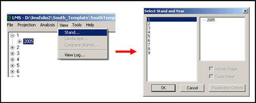Figure 9-5: From the View menu in LMS, you can create an image of a selected stand in a selected year.

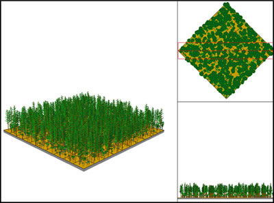Figure 9-6: Stand visualizations can create representative images of your stands from different perspectives. This visualization shows a young loblolly pine plantation.

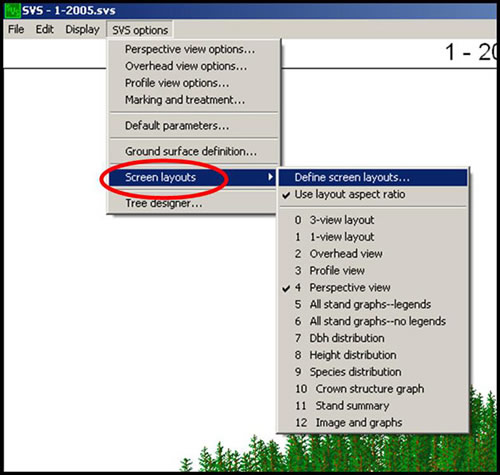Figure 9-7: Within SVS, you can view your stand different ways.

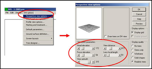Figure 9-8: The Perspective View in LMS simulates an aerial view of the forest. You can use the slider bars in the Perspective View Options to change your viewpoint.

Close that image to return to LMS and now try right-clicking on a year under a stand like you did to open a table specifically for that stand. Select Visualize Stand and notice that the stand and year have already been selected. Click OK. Look at the 3-view layout (0). Notice on the Edit menu on the toolbar there is an option for Copy screen image to clipboard.  If you select this option, you can then paste the visualization into another application such as an image editor, word processor, or Microsoft® PowerPoint. You can also save the visualization as an image file (e.g. as a .BMP file) by selecting the Save File As option from the File menu on the toolbar.

III. “Growing” the stand into the future

Going back to the main LMS window, go to Projection: Stand. Select one of your stands and project it out 50 years (or any number of years that you wish) by selecting the appropriate year under the drop-down menu labeled To (Figure 9-9). You could also do this by right-clicking on the stand and choosing Project Stand from the drop-down menu (just like you can do for tables and stand visualization). Once the stand has been projected, right-click on the last year of your projection (50 years in the future) and select Visualize Stand to bring up a stand visualization for this year. This is an estimate of what the stand will look like in 50 years. Open the summary table for all years and see how the summary statistics are expected to change over time. Note that the trees are expected to get bigger (growth) and fewer (mortality).  You can look at the stand at other points in time as well.

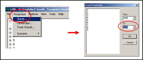Figure 9-9: From the Projection menu in LMS, you can simulate the growth of your stand over time.

Back in the main LMS window, select Tools: Flush entire cache (Figure 9-10). This erases all projections so that you can start over. There is no undo for cache flushes, so make sure you want to start over before selecting that option!

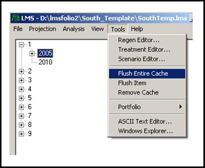Figure 9-10: Flushing the cache will reset your projections back to your original inventory. Be careful – there is no “undo” for his action.

IV.  Do a thinning treatment

Now let us explore some of the real power of LMS.  You will be able to do silvicultural treatments now or in the future and grow out (project) those stands.  For example, have you ever wondered what your stands will look like in 30 years if you did a thinning now or waited 10 years and then did a thinning?  LMS can help you see these differences.

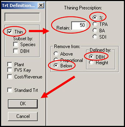
Click the plus next to a stand in LMS so that the year shows. Right-click on the year and select Quick Treatment to bring up the Treatment Definition window. Next click the check box next to Thin, which will expand the prescription portion of the window (Figure 9-11).

We always define thinning by what we retain, not by what we cut. We can choose our retention level in several ways: by percentage of trees retained (%); trees per acre retained (TPA); basal area retained (BA); or Stand Density Index after thinning (SDI). Most of the time we define our retention in terms of TPA, which is the default selection (percentage may also be useful). We can also specify whether we want to thin from below (take the smallest trees and leave the largest), thin from above (take the largest and leave the smallest), or do a proportional thin (select evenly across all diameter classes), and whether we want to rank tree size by height or diameter. A typical thinning would be from below by diameter. If you wanted more diversity, you could thin proportionally. Thinning from above is more difficult, may result in high-grading, and is usually not a good idea.  Consult with a forester if you have questions about the best option for your forest.

Try a simple thinning treatment in which we will keep 50% of the trees and prioritize the largest diameter trees for retention. Type 50 in the Retain field and select the options next to Below, %, and DBH (Figure 9-11). Click OK. Did you hear the chainsaws? Create another summary table. Was your treatment successful?

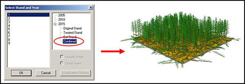
Back in the main portfolio window, click the plus next to the year under the stand you treated to expand it. You will see that there is now an entry for your treatment. Right-click on that year and select Visualize Stand. Notice you have four options now: Original Stand, Treated Stand, Cut Stand, and Combined (Figure 9-12). Try them all.

Go to Tools: Flush Entire Cache (Figure 9-10) so that you can start over with a clean slate. Bring up the Quick Treatment window by right-clicking the year under your stand and selecting Quick Treatment. Click the box next to Thin, but also notice the two boxes under it for selecting a subset by species or DBH. Check the species box, and notice that two new fields appear: Include and Exclude. Use the Include field to specify one or more species to include in your treatment. Likewise, use the Exclude field to specify one or more species to exclude from your treatment. For instance, you may want remove the hardwoods from a loblolly pine stand. Rather than specifying each hardwood species to remove, you could tell LMS to simply exclude loblolly pine and thin everything else to 0 TPA (Figure 9-13). You can specify a species by typing its 2-letter code⁵. Note that when you thin to 0 trees, the other options (above, below, etc.) are irrelevant. Click OK and the treatment is done. On your own, try removing all but one species in your stand.

Figure 9-11: Once you bring up the quick treatment window in LMS, click thin and specify what trees you want left after thinning.

Figure 9-12: After a treatment you can view the original stand, what was cut, what was left, or a combined view.

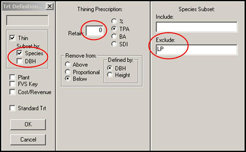Figure 9-13: Under the Thin box in the Quick Treatment window, you can specify a particular species to include or exclude. In this case loblolly pine (LP) is excluded so that this species will be retained while all others (e.g. hardwoods) are removed.

In the example above, everything but one species (loblolly pine) was removed. Suppose we also wanted to thin the remaining species at the same time. You can bring up the Quick Treatment window again in the same year to do an additional treatment. For instance, we may want to cut any remaining trees less than 10 inches in diameter (you may want to change this to something lower if all your trees are under 10”). Click the box for Thin and for subset by diameter (Figure 9-14). Two new fields appear for you to specify a diameter range of trees to be cut: Min and Max. Since we want to cut everything 10 inches and under, type 10 in the Max field and type 0 in the Min field. Since we are retaining 0 trees in this range, leave all other variables as they are and click OK. Click yes to keep the earlier treatment. Run the summary table and do a combined visualization of the treated stand to see your results.

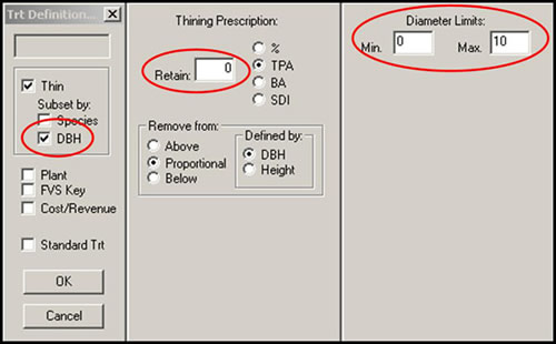Figure 9-14: You can also choose to remove trees only within a certain diameter range.

V. Regeneration

In addition to cutting trees, we can also plant trees (which is especially important after a clear-cut!). In order to plant trees we need a planting file, which is a special file that defines the parameters (species, size, number) of what we intend to plant. The planting file gets cycled in at the next growth cycle (e.g. 5 -10 years) so the planting file needs to be based on what we expect the regeneration to look like when the seedlings are that old.

Go to Tools: Regen Editor (Figure 9-15). On the right-hand side, click Add Regen. Enter the 2-letter species code,5 and the average diameter, height, and crown ratio you would expect the seedlings to be one growth cycle (either 5 or 10 years) after harvesting and planting. Enter the number of stems per acre (your planting density)⁶ and the number of records. The number of records allows the Regen Editor to treat the size parameters you entered as mean values and create a distribution of sizes around those mean values to simulate natural variability. For instance, if you entered 10 records with a mean diameter of 2 inches, you would get 10 slightly different tree sizes that on average have a diameter of 2 inches. Click Save, give the file a name, and save it in your portfolio directory.⁷

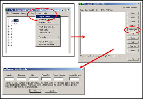Figure 9-15: The Regen Editor allows you to create a Planting File so that you can plant new trees in LMS.

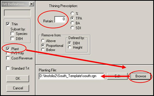
Now let’s try simulating a clearcut with an immediate replanting. First, flush the cache again so that you have a blank slate. Project one of your stands into the future so that it is at least 50 years old. Right-click the year you projected to and bring up the Quick Treatment window. Next, click Thin. Clearcut your stand by leaving 0 trees (since you are leaving 0 you won’t need to change any of the other parameters). Check the box next to Plant and a new part of the form will open up to select a Planting File (Figure 9-16). Click Browse and find the file you just created (which you should have saved in your portfolio directory). Click Open. Now click OK.

Try visualizing the treated stand. What do you see? Recall that the planting file does not take effect until the next growth model cycle, so there should not be any trees. However, project the stand for another cycle and then visualize it and your young trees should appear.

Figure 9-16: Check the Plant box and select your planting file to simulate tree planting in LMS.

VI. Moving on from here

This lesson is not intended as a comprehensive instruction manual for LMS. Rather, it is to familiarize you with some of the most frequently used features of the program and give you a sense of what you can do with the program. There is a lot more to explore in LMS, and there is extensive documentation to help you out along the way. There are two comprehensive sources of help available for LMS:

1. Built-In Help – From the main LMS window, go to Help: Contents to bring up the built-in help program (Figure 9-17). Here you can read about all aspects of the program with step-by-step instructions.

2. LMS Tutorials – There are tutorials available online that will guide you through additional LMS features and functions. These are available at http://lms.cfr.washington.edu/tutorial/.

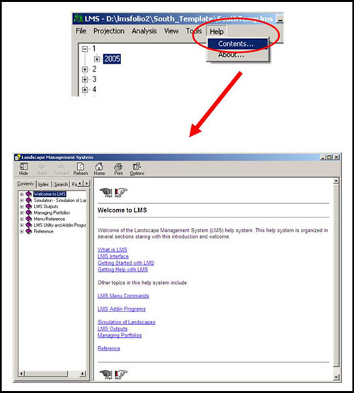Figure 9-17: LMS has a comprehensive built-in help program.

Next Steps:

• There is no quiz for this lesson.
• Go to the Next Lesson.

¹LMS will work with Excel 97 and later, including Excel 2007. Excel 2003 is recommended for best compatibility, though. If you do not have Excel, you can still use many features of LMS, but you will not be able to automatically generate data tables in a spreadsheet. You can still generate tables as text files, though, for use with other programs.

²LMS version 3 is also available, but the procedures in this lesson are specific to LMS version 2 (which is recommended for most family forest applications).

³The text editor option is useful if you do not have Excel or wish to use a different spreadsheet program (e.g. Microsoft Works). If you output the table to the text editor, the information will not be formatted into table columns. You can cut and past the text information into another spreadsheet program and then align the data into table columns by doing a text to columns conversion (consult the instructions with your spreadsheet program for information on this).

⁴For some installations of LMS, an LMS menu may not be added to Excel. You may have to enable the LMS menu by going, in Excel, to Tools: Add-Ins and checking the box next to LMS Excel Utility Functions. If that does not work you can also perform the same autofilter function in Excel by going to Data: Filter: Autofilter.

⁵ A complete list of these species codes for each growth model can be found under “Additional LMS Documentation” in the LMS program group on your computer’s start menu.

⁶Because you are defining what the regeneration will look like 5 – 10 years after you plant, you may want to use a number of trees per acre that is slightly less than what you would actually plant, to account for natural seedling mortality.

⁷Your planting file should be saved in your portfolio directory (e.g. C:\lmsfolio2\your_portfolio\). If it is not saved with your other portfolio files, it may not work correctly.