 |
 |
 |
 |

Working Paper 7
Templates for Forest Sustainability on the
|
|||||||||||||||||||||||||||||||||||||||||||||||||||||||||||||||||||||||||||||||||||||||||||||||||||||||||||||||||||||||||||||||||||||||||||||||||||||||||||||||||||||||||||||||||||||||||||||||||||||||||||||||||||||||||||||||||||||||||||||||||||||||||||||||||||||||||||||||||||||||||||||||||||||||||||||||||||||||||||||||||||||||||||||||||||||||||||||||||||||||||||||||||||||||||||||||||||||||||||||||||||||||||||||||||||||||||||||||||||||||||||||||||||||||||||||||||||||||||||||||||||||||||||||||||||||||||||||||||||||||||||||||||||||||||||||||||||||||||||||||||||||||||||||||||||||||||||||||||||||||||||||||||||||||||||||||||||||||||||||||||||||||||||||||||||||||||||||
Test Stands |
Template |
|||||||||
High Site |
TPA Start |
Best thin age start |
Best thin TPA |
2nd thin age |
2nd thin TPA |
TPA Start |
1st thin age |
1st thin TPA |
2nd thin age |
2nd thin TPA |
High-D* |
350 |
41 |
125 |
15 |
75 |
280+ |
30-40 |
110-135 |
15 |
65-85 |
Med-D* |
220 |
34 |
100 |
15 |
50 |
200-280 |
30-40 |
90-110 |
15 |
65-85 |
Low-D* |
170 |
31 |
100 |
15 |
NA |
<200 |
30-40 |
90-110 |
NA |
NA |
Mid Site |
||||||||||
High-D* |
330 |
54 |
100 |
20 |
50 |
280 |
30-40 |
90-110 |
20 |
45-60 |
Med-D* |
270 |
33 |
150 |
NA |
NA |
200-280 |
30-40 |
90-110 |
NA |
NA |
Low-D* |
170 |
36 |
75 |
NA |
NA |
<200 |
30-40 |
70-90 |
NA |
NA |
*Density |
||||||||||
Most templates involve 2 thinnings but for low density situations only a first thin is applied with further density reductions expected from mortality instead of a second thin. The first treatment should be applied at age 35 with plus or minus 5 years for flexibility. As the site class gets lower one should expect the initial thinning age to increase however the OESF site class range is not large and the test stand treatment results do not suggest that a change to the initial thinning age is needed. The first thinning treatment target would generally leave between 90 to 115 trees (100 TPA) with a slightly higher leave tree target for high site and high density (110 to 135 TPA). A second thinning treatment is appropriate for high sites with medium to high density in as little as 15 years after first entry. For this treatment the leave tree target could be 50 TPA or within a range of 45-60 TPA. For medium site high density a second thinning could occur 20 to 30 years after first entry and leave about 45-60 TPA. The High site low density responded best with only one thin at 30-35 years and a leave tree target of 100 TPA (90-115 TPA range). Less trees (70-90 TPA) were left on the Mid site/low density sites. While the Mid site/medium density stand performed well retaining a higher number of trees, the initial stand condition was closer to DFC than the other test stands.
It should be noted that the first thinnings for biopathways are more aggressive than typical first commercial thins which would likely retain 150-175TPA. While heavier first thins may sacrifice maximum commercial cumulative growth potential, the resulting individual tree growth to accelerate large tree development as well as canopy openings to encourage understory reinitiation are environmentally desirable.
Table of Contents
Click here for the PDF version
List of Figures
| Figure 1: | OESF stands in coarse filter structure classes. See Appendix for structure class attributes. |
| Figure 2: | Trees greater than 32 inches DBH as an Old Forest discriminator. |
| Figure 3: | Large tree stand discrimination for trees greater than 16 inches and 32 inches DBH. |
| Figure 4: | Canopy closure and QMD discrimination. |
| Figure 5: | Canopy closure comparisons |
| Figure 6: | WAC Canopy Closure Thresholds |
| Figure 7: | WAC Size and Density Thresholds |
| Figure 8: | Acceptable and unacceptable stands for TPA, QMD and Ht using a 90% acceptance level. |
| Figure 9: | OESF stands with TPA and QMD for trees > 6 inches DBH |
| Figure 10: | OESF stands with TPA > 24 inches DBH and QMD of largest 40 trees |
| Figure 11: | Percent non-overlapping canopy closure |
| Figure 12: | OESF stands with TPA of trees > 24 inches DBH and canopy closure |
| Figure 13: | OESF stands with TPA of trees > 6 inches DBH and canopy closure |
| Figure 14: | OESF stands with canopy closure and QMD for trees > 6 inches DBH |
| Figure 15: | TPA of trees < 6 inches DBH and the average height of the tallest 100 trees |
| Figure 16: | Average height of 100 tallest trees and QMD for trees > 6 inches DBH |
| Figure 17: | Percent of stands by canopy layers |
| Figure 18: | Assessment with TPA, QMD and CC at 80% acceptance |
| Figure 19: | OESF elevation range |
| Figure 20: | Owl nests present up to 2000 feet. |
| Figure 21: | Dominant species. See Appendix for species abbreviations and data detail. |
| Figure 22: | OESF by site index (SI). Only includes stands for which SI data is available (58%). |
| Figure 23: | Dominant site class ranges |
| Figure 24: | OESF by plant association. See Appendix for data detail. |
| Figure 25: | Young stands (≤ 80 years) by age class |
| Figure 26: | Mid site class test stands |
| Figure 27: | High site class test stands |
| Figure 28: | Mid site class test stand starting points |
| Figure 29: | High site class test stand starting points |
| Figure 30: | Mid site class/high density template visualization |
| Figure 31: | High site class/high density template visualization |
| Figure 32: | Mid site class/medium density template visualization |
| Figure 33: | High site class/medium density template visualization |
| Figure 34: | Mid site class/low density template visualization |
| Figure 35: | High site class/low density template visualization |
| Figure 36: | TPA and QMD for trees > 6 inches DBH |
| Figure 37: | TPA for trees > 6 inches DBH and canopy closure |
List of Tables
| Table 1: | Outcomes by acceptance level |
| Table 2: | Mid site class/high density scenarios |
| Table 3: | Mid site class/high density results comparison |
| Table 4: | High site class/high density scenarios |
| Table 5: | High site class/high density results comparison |
| Table 6: | Mid site class/medium density scenarios |
| Table 7: | Mid site class/medium density results comparison |
| Table 8: | High site class/medium density scenarios |
| Table 9: | High site class/medium density results comparison |
| Table 10: | Mid site class/low density scenarios |
| Table 11: | Mid site class/low density results comparison |
| Table 12: | High site class/low density scenarios |
| Table 13: | High site class/low density results comparison |
| Table 14: | Summary of template pathways |
| Table 15: | Test stands to template |
Introduction
The Olympic Experimental State Forest (OESF), managed by the Washington State Department of Natural Resources (DNR), was established to allow experimental forest treatments in order to provide habitat and biodiversity values, i.e. environmental stewardship, while sustaining harvest activities for the highest possible economic return to the trust beneficiaries. A Habitat Conservation Plan (HCP) covering all state forestlands in western Washington inherently raises the burden of proof that experimental silviculture treatments conducted on the OESF shall meet the commodity production and ecosystem conservation objectives identified within the HCP. That burden presents planning and performance assessment hurdles for both the environmental and economic analysis of any management strategy.
A process to assess habitat conditions and economic viability relative to acceptability thresholds for a variety of site conditions was developed in prior research to evaluate riparian buffer effectiveness for achievement of mature conifer forest characteristics along streams (Gehringer 2006, Zobrist et al 2004). This assessment methodology was shown to be useful for iterative development of management pathways to effectively produce desired future conditions (in this case old forest attributes). Once pathways are identified, treatments are linked to forest types and transformed into management templates for easier implementation. Such management strategies have become known as biodiversiity management pathways or biopathways (Carey et al 1999). Several key features characterize biopathways including periodic thinnings, long rotations, and supplementary attention to legacy features including snags, downed logs, and understory hardwoods. When biopathways are incorporated into a series of management templates for stand level treatments, they can provide easy-to-use implementation guidelines for forest managers, regulatory agencies, and policy-makers, resulting in a substantial savings in time and cost. Simulated treatments can also be extended to the landscape level for integration of spatial and temporal considerations in support of forest planning. The purpose of this project was to determine if extending this assessment process for development of forest management templates for the OESF could enhance achievement of the economic and environmental objectives identified by the DNR in the HCP.
This paper briefly reviews the scientific approach that is being employed, and starts the analysis by identifying the desired future stand conditions and analyzing the differences between forest structure stage classification systems. We then establish performance thresholds for the assessment of both old forest conditions and economic performance. We consider and evaluate a large range of biodiversity pathways, selecting those with the best joint economic and old forest structural performance. We consider fine filter options to narrow the range of selection among the better management pathways. We categorize the different stand types in the forest and identify those that would be most plentiful and productive as candidates for management templates. Finally we discuss the findings, characterize the robustness of the templates by analysis of the test stands, and offer summary conclusions.
Scientific Approach and Methodology
The Rural Technology Initiative (RTI) at the University of Washington, College of Forest Resources has pioneered the development of a non-parametric, multivariate, statistical assessment process for use with the Landscape Management System (LMS) to rigorously evaluate whether the stand structures produced by management pathways will result in desired forest structural conditions defined by a target set of forest stand inventories (Gehringer 2006). This assessment process has been used to construct templates to assist in the development and implementation of management treatments to achieve desired forest conditions (DFC) along streams in the Pacific Northwest and to restore old forest habitats in the US Southeast (Zobrist et al. 2005a&b).
LMS is an evolving computer-based, landscape-level forestry analysis software tool developed at the University of Washington, College of Forest Resources in partnership with Yale University (McCarter et al. 1998, McCarter 2001). LMS offers a software platform for the integration of component capabilities that include growth and yield models, interactive stand treatment simulation programs, tabular and graphical analytical outputs, and stand and landscape visualization programs. Data sources necessary for LMS include stand inventory information (tree-based measurements), landscape data (slope, aspect, elevation, site quality), and Geographic Information System (GIS) spatial data (stand boundaries, streams, roads, etc.). LMS can be used to project stands and landscapes forward in time to predict potential future stand and landscape forest conditions, while virtually treating stands through harvesting, regeneration, and other activities to simulate potential management practices. More information and software downloads are available from the LMS web site at http://lms.cfr.washington.edu .
For this investigation, the PN ( Pacific Northwest) variant of the Forest Vegetation Simulator (FVS) was selected for use as the tree growth model within the LMS projection framework. FVS has been developed by the USDA Forest Service as an individual-tree, distance-independent growth and yield model. The PN variant of FVS is the only publicly available growth model that will simulate growth and yield for all major forest tree species, forest types, and stand conditions found within the OESF. More information and a suite of FVS regional variants are available for download at no charge from the USFS web site at: http://www.fs.fed.us/fmsc/fvs/.
Thresholds of acceptability have been evaluated both for forest functionality, based on the similarity of forest structure to that of existing forests with known environmental attributes, and also for economic viability, based upon comparative rates of return. These thresholds aid in the selection of preferred management strategies for meeting environmental and economic goals, which are then translated into management templates. Management templates provide a series of treatment guidelines that facilitate simple and flexible implementation of forest practice activities for typical initial forest conditions. They provide tools for the creation of preferred outcomes at the stand level over time that can further be extended to characterize a mix of stand conditions at the landscape level.
While this assessment procedure and application is relatively new, both the statistical and economic analysis methodologies are well-established and have been peer-reviewed in the work cited above. Applications of this work, within the context of this project, include developing experimental pathways for the OESF, establishing acceptable riparian management pathways under the HCP, and becoming a building block in the strategic planning development process for upland and riparian management objectives within Pacific Northwest forests managed by the DNR. Visual displays have been developed to demonstrate post-treatment stand structures and to help explain the statistical procedure to foresters and stakeholders.
Step 1: Identifying the desired stand conditions
The conservation objective for the OESF as stated within the DNR HCP (1997) is to:
“Develop, implement, test, and refine management techniques for forest stands that integrate older forest ecosystem values—including the stands’ functioning as dispersal, foraging, roosting and nesting habitat for spotted owls – with commercial objectives for those stands.”
A supplementary part of the conservation strategy is stated as:
“A principle working hypothesis of the OESF is that landscapes managed for a fairly even apportionment of development, from stand initiation to old growth (Oliver and Larson 1990) will support desirable outputs of both commodities and ecosystems functions.”
The forest type in shortest supply as a consequence of past commercial management practices has been identified to be that of old conifer-dominated forests. As a result, increasing the acreage with older forest attributes is an important objective for the DNR. Not surprisingly, the concept of intentionally managing stands to accelerate development of old forest attributes using treatment strategies known as biopathways (Carey et al 1999, Lippke et al 1996) has become a focus of DNR management planning for the OESF.
The first step in creating a management template is to identify the forest management outcomes desired on the OESF. Two approaches are useful for determining management direction once desired outcomes are identified. The first approach has been designed to aid in development of a specific structure or forest condition as a surrogate for a suite of ecosystem functions. Specific HCP thresholds have been specified by DNR requiring:
- “Harvest activities will maintain the proportion of old forest habitat at or above 20 percent of each landscape planning unit and will not reduce sub-threshold proportions.” and…
- “Plans for harvest of young or old forest habitat will recognize the importance of interior old forest conditions to overall ecosystem function and will maintain or develop these conditions in accordance with landscape plan.” ( DNR 1997, Hanson et al. 1993)
These thresholds are not intended to be targets for management; rather, they are considered minimum acceptable objectives.
The second approach is a more “fine filter” approach of managing for specific, individual functions such as canopy closure, snags, or large woody debris (LWD). Templates are first developed based on managing for a statistically acceptable desired structure and then refined as appropriate with the fine filter approach for addressing specific functions believed to be critical as part of the template validation. Many of these additional functions are so variable in old forests that they may not provide useful discrimination properties as to whether a stand has achieved older forest characteristics or not but the parameters may still be important for certain desired outcomes.
Old forest conditions on the Westside are considered functionally adequate for many species at risk (Franklin and Spies 1991). These forests have been modeled in prior studies using samples of old forests taken from Forest Service Forest Inventory and Analysis (FIA) data (Gerhinger 2006). For this study we have detailed inventory data that has been provided by DNR for all the stands in the OESF. Stand inventories were sorted by age and examined to better understand the discriminating features of those forests classified as being older than 80 years, a temporal threshold at which western Washington forests begin to exhibit mature forest characteristics (DNR 2005). The DNR also provided inventory data representative for most all OESF forest areas that have historically supported successful northern spotted owl ( Strix occidentalis caurina) nests as a subset of stands with major environmental importance. A total of 3492 inventory plots were examined of which 2825 plots were found to be forests less than or equal to 80 years old, 658 plots were found to be forests older than 80 years, and 9 plots were sites that had supported successful owl nests (Horton pers. com.).
For development of an assessment procedure, a sample dataset is established from actual inventories of forests considered representative of the desirable forest condition (DFC). This dataset is referred to as the target dataset. Once a sufficiently representative dataset has been identified, a nonparametric assessment procedure can be used to statistically discriminate whether a forest stand has structural characteristics that are similar to or different from the target database (Gehringer 2006).
The goal of developing a management template is to select site-appropriate biodiversity pathways that will move stands on a trajectory towards the old forest structure target while generating revenue for the trust beneficiaries. Best performing pathways are identified as those that achieve the old forest structure target quickly while maintaining economic viability by generating periodic harvest revenues.
Key questions that must be addressed are how to define and measure the “DFC” target; what sites to develop templates for; and what starting conditions to use for developing templates.
Defining and measuring the DFC
There have been several different “coarse filter” structural stage classification systems developed for western Washington (Oliver and Larson 1990, Carey et al 1996) in addition to codified definitions such as the WAC definitions of habitat (nesting roosting and foraging, dispersal, young mature marginal etc). All of these systems were developed by a somewhat limited analysis of actual stand conditions relative to observed habitat during the early years of interest in protecting northern spotted owl habitat and ecologically valuable old forests. Historical “coarse filter” approaches for structural stage identification should be distinguished from statistically robust assessment methods. In the OESF, we have more and better empirical data on stands than was available when these classification systems were developed (see appendix). Data currently available for the OESF includes stand inventory information for one-time productive owl nests and stands defined to be of a certain age category such as all stands with dominant trees that originated in 1925 or earlier. We have identified these stands as a useful class for developing a functional target. Stands that are older than 80 years, a benchmark frequently cited in literature as a transition point to older forest conditions (Franklin et al. 2005) include the “21 blow” stands on the OESF which are known to provide substantial diversity in structure (Commission on Old Growth Alternatives for Washington’s Forest Trust Lands 1989).
An important question is how well do actual nest stands and age thresholds correlate with various historic old forest habitat measures?
Structure Class Characteristics
Figure 1 shows the distribution of OESF old forest stands greater than 80 yrs, owl nest stands (only 9 that were once productive), and all other forest stands across a simple 4-stage structure classification (see appendix) parameterized in the Landscape Management System (LMS). The distribution demonstrates a high correlation between owl nests and old forests with a poor fit with other forests validating the conceptual underpinnings of the structure classification process. Note the single owl nest in Stand Initiation structure class. This stand is an outlier that is the result of a fairly open condition with a few large trees that, given the course resolution of this stand classification, is lumped along with the other open stands and not with the other older stands; an imperfection in the algorithm discrimination characteristics.
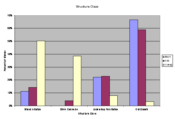 |
Figure 1. OESF stands in coarse filter structure classes. See Appendix for structure class attributes. |
Most structure classification systems rely on the number of big trees per acre as the most important discriminating factor for old forests. In the case above, big trees are considered to be greater than 32 inches diameter at breast height (DBH). Figure 2 shows that the historic threshold of more than 6 trees greater than 32 inches DBH (Oliver and Larson 1990, see appendix) certainly assures that the forests are old (older than 80yr) although it excludes some old forest stands and some owl nests with fewer than 6 big trees. Figure 2 also demonstrates that canopy closure does discriminate to a degree both owl nests and old forests, especially when used with large trees as a second defining variable.
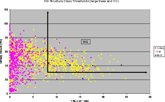 |
Figure 2. Trees greater than 32 inches DBH as an Old Forest discriminator |
Figure 3 looks at overstory and understory with the number of trees that are 16 inches minimum diameter shade tolerants on the y axis and trees that are 32 inches minimum diameter in the overstory on the x axis. The range of trees greater than 16 inches is quite wide providing less discrimination than canopy cover when used along with big overstory trees.
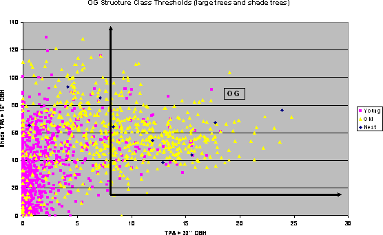 |
Figure 3. Large tree stand discrimination for trees greater than 16 inches and 32 inches DBH. |
Figure 4 shows how canopy closure and the quadratic mean diameter of the largest 40 trees discriminate between Stand Initiation structures and Stem Exclusion structures as well as how the larger diameter and older trees that are considered as having more diversity have diverged from the trend growth of young stands. The normal growth progression of stands from low canopy closure and low QMD to high excludes many of the old forests which have higher QMD even at lower canopy closure. Some of these stands may be inappropriately classified with young open stands as Stand Initiation structure if neither age or diameter are used as discrimination parameters.
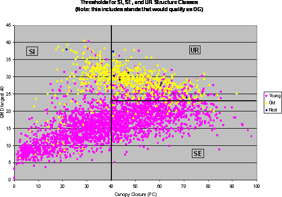 |
Figure 4. Canopy closure and QMD discrimination. SI = Stand Initiation, SE = Stem Exclusion, UR = Understory Reinitiation |
Canopy closure measures have evolved over time and the currently preferred non-overlapping or open sky gap measure does not correlate well with equation-derived methods developed for some of the earlier Habitat Conservation Plans (Figure 5). The non-overlapping definition developed by Crookston and Stage (1999) for use with FVS is used for this analysis and is the calculated as the projected crown basal area from all trees as a percentage of an acre corrected for crown overlap. However, canopy closure for the structure classification algorithm is derived from regression equations developed with data from Plum Creek Timber Company Habitat Conservation Plan (Oliver et al. 1995) and programmed into LMS (hence the above abbreviation PC). Canopy closure estimation and associated light and vertical profiles with implications for important habitat attributes, such as understory vegetation development, is an area of research where more work is needed.
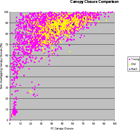 |
Figure 5. Canopy closure comparisons |
Several coarse filter definitions have been codified in regulations. The Washington Administrative Code (WAC) description of old forest habitat (WAC 222-16-085; see appendix) requires a canopy closure of 60% or more and a layered, multispecies canopy where 50% or more of the canopy closure is provided by large overstory trees (typically with 75 trees greater than 20 inches DBH per acre or at least 35 trees per acre greater than 30 inches DBH). Figure 6 demonstrates that the first part of the WAC definition involving canopy closure does provide discrimination of old forests in the OESF.
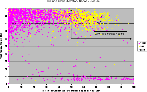 |
Figure 6. WAC Canopy Closure Thresholds |
However, part 2 of the definition requiring 75 trees greater than 20 inches DBH or 35 trees greater than 30 inches DBH per acre produces almost an empty set of stands and with no owl nests. OESF forest data suggests that in recent history these forests have not produced that many big trees or that much density.
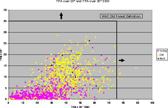 |
Figure 7. WAC Size and Density Thresholds |
Step 2: Selecting the variables for discrimination in the OESF
A variety of combinations of management oriented variables, were evaluated to determine those that best discriminate the target forests from all others (see appendix and figures 1-17). Based on other studies a high degree of discrimination is expected using trees per acre (TPA) and quadratic mean diameter (QMD) with canopy closure and average height potentially important (Gehringer 2006). The n-dimensional plot of these selected variables represents a joint empirical distribution of key variables that provides the basis for the assessment of whether a treated stand is similar to or different than the target stands used to define old forests.
Once a target dataset is identified that represents the distribution of desired forest conditions, an acceptance region may be defined within that dataset based on probabilities derived from a probability density function (PDF, see figure 8 below). The definition of such an acceptance region must take into account two factors. First, the acceptance region should contain the most likely values, those near the mode and having the largest PDF values. Second, the extent of the acceptance region should be controlled by the distribution of the desired forest conditions within the target dataset and be specified by the probability defined by the acceptance region. These two objectives are met simultaneously by choosing an acceptable level of error (analogous to the selection of an alpha-level in the classical statistical hypothesis testing context) specifying the probability of not being in the acceptance region. If we let p be the probability of not being within the acceptance region, or the probability of error, then the probability of being within the acceptance region is given by 1-p. The contour of the PDF containing (1-p)100% of the probability identifies the critical contour of an acceptance region for the desired forest conditions, relative to the target dataset.
This procedure will determine whether the stand parameters are or will be (after management simulations) within the acceptance region for the desired acceptance level (1-p)100%. If the stand parameters are within the critical contour, then they are statistically indistinguishable from the target acceptance region at the (1-p)100% acceptance level and are considered acceptable (within the target range of variability). If the stand parameters are outside the critical contour, then they are statistically different from the target acceptance region at the (1-p)100% acceptance level and are considered unacceptable. An illustration of such a plot is taken from Gehringer (2006) showing that of the observed old forest target stands portrayed in three dimensions, when the acceptance level is set at 90% about 10% of the stands that appear to be outliers are rejected. Setting the acceptance level lower restricts acceptance to those stands closer to the central mode, resulting in a tighter target.
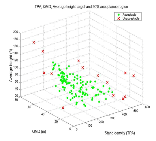 |
Figure 8. Acceptable and unacceptable stands for TPA, QMD and Height using a 90% acceptance level (Gehringer 2006) |
Since the number of owl nest sites was so small, we selected the 80-year age filter as a reasonable set of target stands that appear highly correlated with desired conditions in the WAC and HCP, as well as actual nest plots.
From a purely statistical perspective, TPA and QMD for trees greater than 6 inches DBH provides a very tight cluster of old forests relative to other forests as described by OESF plots older than 80 years and the owl nests are further clustered in the middle of the old forest cluster for OESF stands (Figure 9). These metrics have often been linked to owl biology and old forest structures in riparian studies and are directionally in alignment with the WAC structure stage thresholds. Basal area or other density measures are not suitable as they can represent very disparate stand conditions such as high TPA with low QMD or the opposite producing the same measure (RTI 2001). Canopy closure has also been considered important to owl biology and is an important metric in the WAC definition.
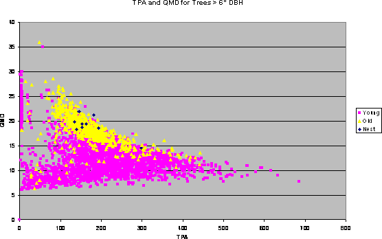 |
Figure 9. OESF stands with TPA and QMD for trees > 6 inches DBH |
Canopy layers have been considered important in the owl literature and certainly can be used as a part of a fine filter. An algorithym to differentiate canopy layers developed for use with LMS by Baker and Wilson (2000) has been used for this analysis. In figures 10-17 we evaluate a range of variables providing evidence of their behavior in contributing to old forest stand discrimination.
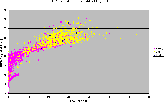 |
Figure 10. OESF stands with TPA > 24 inches DBH and QMD of largest 40 trees |
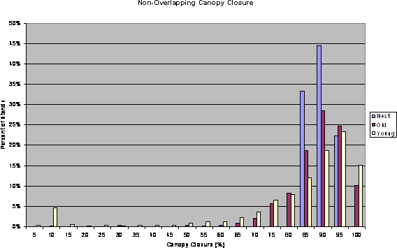 |
Figure 11. Percent non-overlapping canopy closure |
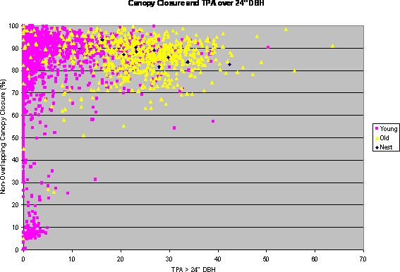 |
Figure 12. OESF stands with TPA of trees > 24 inches DBH and canopy closure |
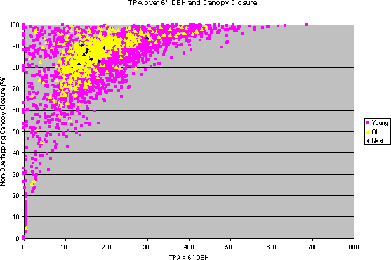 |
Figure 13. OESF stands with TPA of trees > 6 inches DBH and canopy closure |
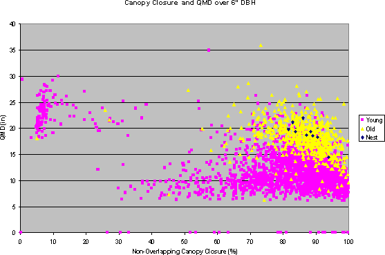 |
Figure 14. OESF stands with canopy closure and QMD for trees > 6 inches DBH |
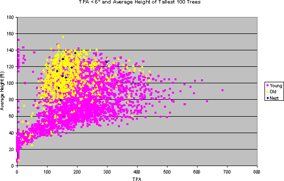 |
Figure 15. TPA of trees < 6 inches DBH and the average height of the tallest 100 trees |
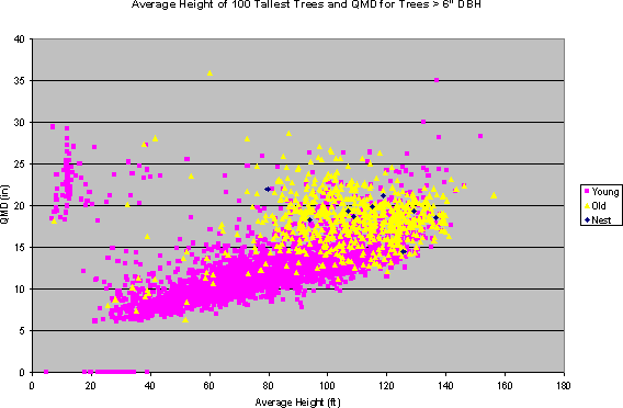 |
Figure 16. Average height of 100 tallest trees and QMD for trees > 6 inches DBH |
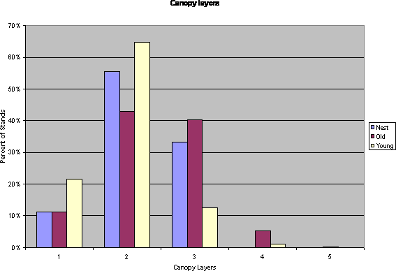 |
Figure 17. Percent of stands by canopy layers |
In figure 10, we note that the number of large trees and the QMD of the largest trees are highly correlated. In figure 11, we note that the correlation between owl nests and old forests is very high, however the owl nests are concentrated with a much narrower distribution between 85-95% canopy closure such that either too much canopy closure or too little is rejected. The comparison of large trees and canopy closure, shown in figure 12, indicates that there is a large variation in the large trees with little discrimination. When TPA for trees greater than 6 inches DBH are shown in Figure 13 with respect to canopy closure, we note a much smaller cluster for old forests and owl nests. In figure 14, we note substantial discrimination using QMD for trees greater than 6 inches DBH and canopy closure. In figures 15 and 16, old forests, owl nests, and young forests appear to have little discrimination by height. In figure 17, we note no clear trend in canopy layers other than forests that are 80 years and younger tend to have less than 3 layers suggesting no utility in including canopy layers as a discriminating variable.
In summary, TPA and QMD are important discriminators with canopy closure a potential third variable. When these variables are restricted to only larger diameter thresholds, such as trees per acre greater than 20 inches DBH, results show thresholds that range all the way from zero to the upper limit, which reduces the power of discrimination. Hence it is difficult to improve upon the TPA and QMD for trees 6 inches DBH and larger as the dominant discriminators as shown by the tight clusters in Figure 9.
Step 3: Establishing performance thresholds
The next step is to establish specific performance thresholds relative to the targeting and assessment procedure described above. This requires establishing minimum temporal performance criteria against which potential management alternatives can be compared at the selected acceptance level. We can then define our performance metric as the percentage of time (using modeled stand growth with treatment simulations on 5-year increments) over an extended period (100 years, for example, coincides with the maximum period of the DNR HCP) that a resulting forest structure is likely to fall within the target region at a determined acceptance level. The speed with which a forested area achieves the desired condition and the duration that the forested area stays within the desired condition for any management alternative become measures of achievement for the future forest condition.
Using a three variable target:
TPA of trees > 6 inches DBH
QMD of trees > 6 inches DBH
Non-overlapping canopy closure
Acceptance |
Nest |
Old |
Young |
80% |
89% |
80% |
18% |
85% |
89% |
85% |
26% |
90% |
100% |
90% |
37% |
And setting the acceptance level at 80%, 85% or 90% where 100% acceptance would include all target stands, we note that we successfully include 89% of the nests, 80% of the old forests and reject 82% of the young forests defining our target with 80% acceptance (table 1 and figure 18). The 18% of the stands that are not rejected are predictably older stands just a few years younger than our arbitrary 80 year threshold. The fact that we have not rejected all young stands is to be expected.
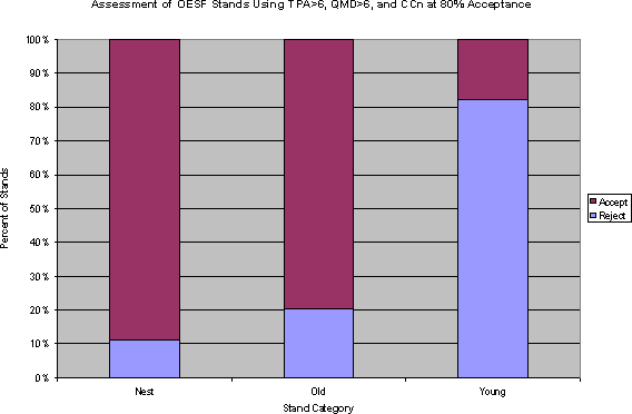 |
Figure 18. Assessment with TPA, QMD and CC at 80% acceptance |
An economic performance threshold is also necessary for selecting preferred management alternatives. Two measures of economic performance are relevant: forest value and bare land value (Klemperer, 1995). Forest value (FV) represents the total economic value of a forest based on how that forest is to be managed. Bare land value, also called soil expectation value (SEV), is the component of forest value representing the land exclusive of any existing timber. SEV represents the net present value of reinvesting land in forest management after the existing timber has been harvested. SEV is most closely related to the long-term economic performance of forest management and may be the most relevant single measure for assessing the economic sustainability of potential templates. To establish a specific performance threshold based on SEV, the minimum acceptable rate of return (MAR) at which SEV is to be evaluated must be considered. We use a 5% discount rate for determining SEV consistent with many other forest economics assessments involving state lands. Since an examination of management alternatives for the existing stands in the OESF will be more useful for this investigation than simulations of theoretical stand regeneration, we ignore the initial investments in forest regeneration as sunk costs and simply compute the Net Present Value difference across our management alternatives starting with current stand inventories and taking into consideration all future treatment costs and revenues.
Step 4: Generating alternatives
The next step is to generate a set of alternatives that will be assessed relative to the established performance thresholds. A literature review provides strategies that may be able to achieve the desired stand conditions while meeting economic performance targets. For example, given a goal of complex structure typical of old-forest conditions, Carey et al. (1999) and Lippke et al. (1996) demonstrated management strategies referred to as “biodiversity pathways” that have been designed to achieve old forest structure while generating a favorable economic return. The DNR Environmental Impact Statement (EIS) for the preferred alternative to establish the Sustainable Harvest Calculation (SHC) has incorporated “biodiversity pathways” to accelerate the restoration of habitat associated with old forest functionality. With biodiversity pathways as a basis, a series of potential silvicultural alternatives for development of management templates were established for use on the OESF. In particular we investigate the ability of one, two, or three thinnings with variable retention densities and timing as representative of a range of biodiversity pathways. Different strategies will be needed to address different site classes, as growth rates and windows of opportunity for thinning will vary. This means that a set of templates, rather than an individual template, will be necessary to cover a range of site conditions. Stand conditions that merit the development of independent management templates require identification.
Step 5: Identifying stand conditions appropriate for templates
The goal of this investigation is to develop templates that cover a range of initial stand conditions commonly found in younger OESF stands. Key stand level variables that logically suggest different templates include elevation, dominant species, site index, plant association, habitat type, and age class. Figure 19 shows that most of the OESF stands are below 1000 feet above sea level although, as noted in Figure 20, there are a few owl nests above 2000 ft. Figure 21 shows that the dominant species include western hemlock (Tsuga heterophylla), shown as WH, and Douglas-fir (Pseudotsuga menziesii), shown as DF, mixed with WH. Figure 22 shows OESF site quality based upon 50-year western hemlock and Douglas-fir site index calculations. Most of the OESF can be categorized into two site class ranges as shown in Figure 23. Nigh (1995) developed a formula to convert between DF and WH site indexes. Nigh’s conversion was used here to identify a High site index mode as 120WH or 135DF and a Mid to High index mode as 105WH and 120DF. These site classes capture most of the OESF stands in two ranges for which we can develop templates and determine their validity.
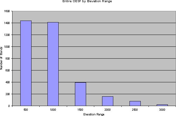 |
Figure 19. OESF elevation range |
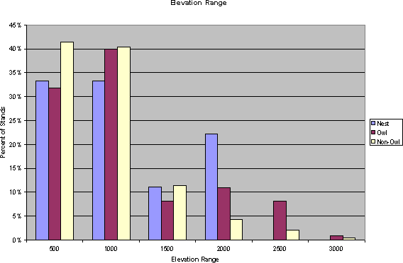 |
Figure 20. Owl nests present up to 2000 feet. |
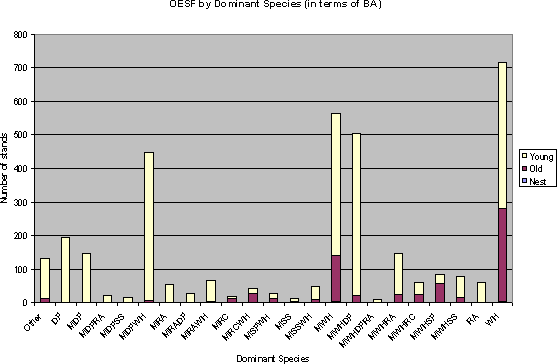 |
Figure 21. Dominant species. See Appendix for species abbreviations and data detail. |
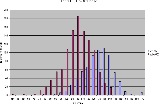 |
Figure 22. OESF by site index (SI). Only includes stands for which SI data is available (58%) |
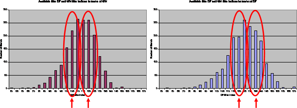 |
Figure 23. Dominant site class ranges |
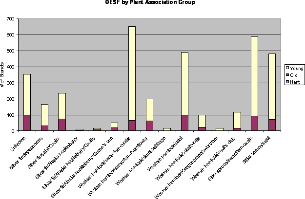 |
Figure 24. OESF by plant association. See Appendix for data detail. |
Figure 24 shows that 63% of the OESF falls within 4 plant association groups (PAGs). PAG assignments are provided by the data and are be used within LMS to refine the growth model behavior for simulations. Figure 25 characterizes the number of stands that are less than or equal to 80 years old by age suggesting that there are a large number of stands in the 25-40 year ranges and that this age may be an appropriate age to initiate treatment.
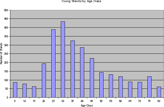 |
Figure 25. Young stands (≤ 80 years) by age class |
By further subdividing the stands in these site class ranges by density (figures 26 & 27), we can evaluate treatment options for their suitability. The three stands covering a density range are located on the TPA/QMD chart for the Mid site class stands in figure 28 and for High site class stands in figure 29. Stands, generally in the 30-year age range, are considered quite suitable for a commercial or biopathway thinning treatment.
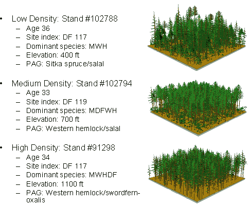 |
Figure 26. Mid site class test stands |
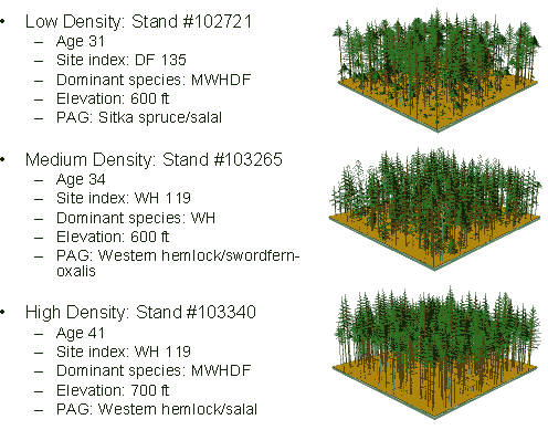 |
Figure 27. High site class test stands |
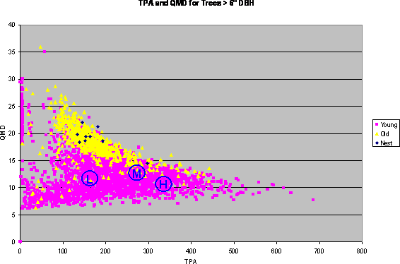 |
Figure 28. Mid site class test stand starting points |
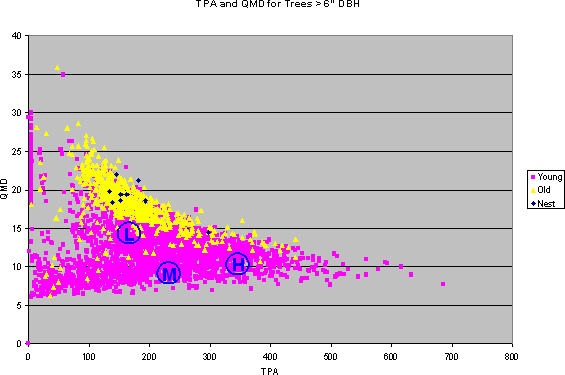 |
Figure 29. High site class test stand starting points |
Step 6: Testing alternatives
Alternative treatments to these representative test stands are evaluated using the projection and simulation capabilities of the Landscape Management System (LMS, http://lms.cfr.washington.edu/lms.php). LMS is a forestry software package developed at the University of Washington that provides access to a number of regional singletree growth models as well as visualization and spatial models (McCarter et al. 1998, McCarter 2001). LMS tracks changes to tree list inventories through growth and treatment simulations. Analytical outputs include stand structure changes and costs for each growth period (in this case 5 years is the growth period). When harvest activities are simulated, a log merchandising algorithm provides analysis of harvest volumes linked to a number of other associated environmental and economic metrics including revenues, disturbance hazard, carbon storage, and habitat suitability indices.
At 5-year growth intervals for each simulation throughout the duration of the period of interest, the three key stand variables (TPA, QMD, and canopy closure) are computed within LMS and the assessment procedure is applied to determine the number of growth intervals that the stand of interest is in or out of the target region for a given management alternative. NPV per acre is calculated based on merchantable volume outputs in thousand board feet (MBF) from harvest simulations with gross revenue estimates adjusted for treatment-specific logging costs discounted to the initiation time point with a 5% real discount rate. Department of Revenue stumpage value estimates (DOR 2006) were used with Area 1 & 2 values for first and second quarters of 2006 averaged across haul zones 2 & 3 with stumpage values adjusted for costs based on:
- -$100/MBF for 5 MBF volume yield per acre; typical of a first thinning,
- -$35/MBF for 5-10 MBF volume per acre; typical of a second or later thinning
- -$15/MBF for 1-30 MBF volume per acre typical of a second or third thinning or less than scale operation
- $0 adjustment for >30 MBF, a typical scale harvest rotation
The environmental and economic results of each alternative can be charted relative to the minimum acceptable performance thresholds. The results of tested alternatives may reflect a wide range of performances, with some meeting neither the desired future condition or economic performance thresholds, some meeting one but not the other, and others that meet both. Those alternatives that meet both the economic and environmental criteria will be considered as viable template options.
More than 75 alternative treatments were considered but many were eliminated as not acceptable. For example the first set of up to 3 thinnings with final harvest in 65 years (begin age of 35 years) at approximate age 100 were thinned from below for all trees >6 inches DBH. This treatment not only thinned the smaller overstory trees, but also removed understory trees >6 inches DBH resulting in insufficient lower canopy layers following later thinnings required to meet the stand structure target. By thinning >6 inches DBH for the first thinning, >12 inches DBH for the second thinning and >15 inches DBH for the third thinning much better achievement of time in the target was obtained. The thinning alternatives were designed to evaluate both the timing of a second thinning and the impact of number of trees retained in the first and second thinning. While the dominant treatment impact is thinning, other available legacy attributes would also be retained such as snags and downed logs. A total of 26 biopathways and two control treatments were simulated with results presented below.
High density stands
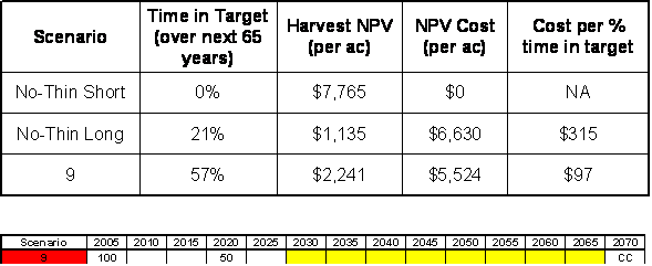
Two control treatments and 26 treatment alternatives with time of thinning and TPA retained are illustrated in table 2, for the Mid site class/high density subset of stands. The darkened area shows when the stand passes the assessment test as not being different than the old forest target. Scenarios 6, 9, and 47 are highlighted as having extended time in the target zone and respectable economic performance as summarized in table 3 along with the No-Thin Short and Long rotation controls for comparison. The No-Thin Short rotation simulates an approximate optimal economic commercial rotation while the No-Thin Long rotation provides a comparison to no action until year 2070, an approximate age of 100 years for recycling the management pathway. As noted on table 3 there is a trade-off between high NPV for Scenario 9 although lower time in target than Scenario 6 or 47. The NPV cost (lost revenue) is much higher for the No-Thin Long alternative than for the biopathways.
| Table 2. Mid site class/high density scenarios |
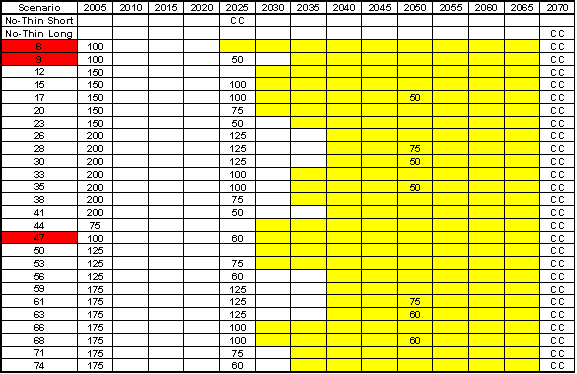 |
| Table 3. Mid site class/high density results comparison |
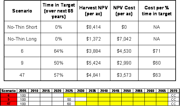 |
The marginal cost per time in target (last column) provides a joint efficiency metric for fairly similar alternative performance simulations. The No-Thin Short rotation provides a commercial benchmark for economic comparison. Scenario 9 has the lowest cost per % time in target at $60 per % time in target and hence if replicated can produce the lowest cost per number of acres in target. However, Scenario 9 also has the lowest time in target which suggests that more treated acres might be needed to meet a landscape target. The No-Thin Long treatment alternative which did not reach the target by 2070 and produced no harvest revenue can be regarded as the worst case. While Scenario 9 produces an NPV of $5424/acre, this may barely make a target SEV for sustainable management at 5% rate of return. Factoring in estimated regeneration costs and annual administrative costs appear to lower the SEV to nearly zero. Since the SEV is quite sensitive to management efficiency issues beyond the scope of this study, we have limited the economic analysis to an NPV of net future revenues for the rotation (including a second rotation for the No-Thin Short scenario resulting in comparable time intervals).
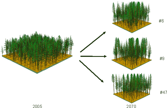 |
Figure 30. Mid site class/high density template visualization |
While the visual appearance of Scenario 9 appears to show slightly fewer trees at 2070 the difference is not substantial (figure 30). The stands look similar and all have extended time in the target zone.
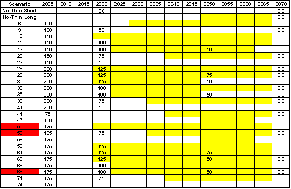
| Table 4. High site class/high density scenarios |
 |
| Table 5. High site class/high density results comparison |
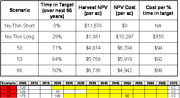 |
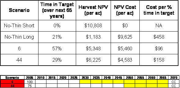
For High sites and high density the results shown in table 4 and 5 and figure 31 are quite similar, however the time in target is longer and is reached more quickly; as little as 15 years after the first thinning and the second thinning is moved up to 2020 instead of 2025. The No-Thin Long scenario still performs poorly although reaching the DFC target about 30 years later than the thinned scenarios. When compared to a commercial rotation (No-Thin Short), Scenario 53 has NPV costs of $5919 per acre with a marginal cost of $92 per % time in target, about 50% higher than for the Mid site class for comparable high density. In this case the lowest cost scenario (68) is not the lowest marginal cost scenario (53).
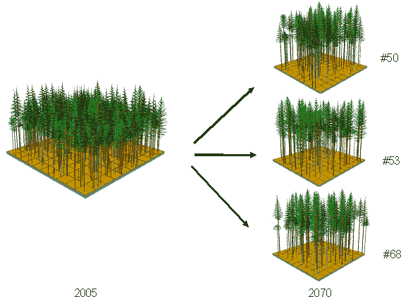 |
Figure 31. High site class/high density template visualization |
Even in these high density scenarios, the alternatives with two thinnings performed better than the three thin alternatives.
Medium density stands
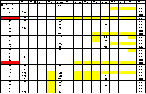
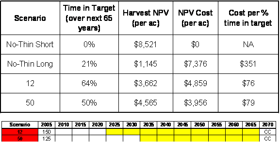
The Mid site class and medium density stand is already closer to the DFC than the high density stand and there are fewer treatments that are effective with less that can be removed. Only one thinning is needed to approach the greatest time in target. While Scenario 50 results in the lowest cost (NPV $3956/acre) and removes a few more trees in the first thinning, the marginal cost is slightly higher than Scenario 12 at $76 per % time in target (table 6 & 7 and figure 32). With less density these stands are more sensitive to thinning treatments. The marginal costs are slightly higher for the Mid site/medium density treatments than for the Mid site/high density but lower than for High site/high density stands.
| Table 6. Mid site class/medium density scenarios |
 |
| Table 7. Mid site class/medium density results comparison |
 |
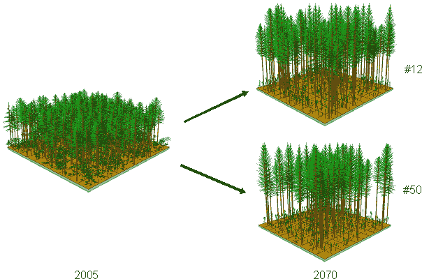 |
Figure 32. Mid site class/medium density template visualization |
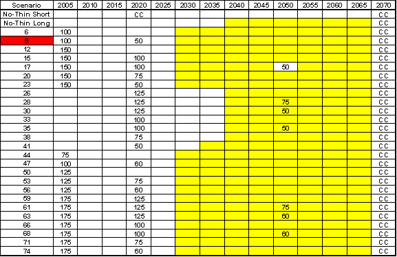
For the High site class and medium density stand the first thinning can be moved up 5 years to 2020 without diminishing NPV or time in DFC. The cost for the best scenario with two thinnings is $5524/acre, with a relatively high marginal cost of $97 per % time in target (table 8 & 9 and figure 33).
| Table 8. High site class/medium density scenarios |
 |
| Table 9. High site class/medium density results comparison |
 |
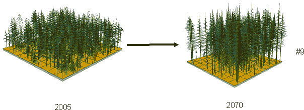 |
Figure 33. High site class/medium density template visualization |
Low density stands
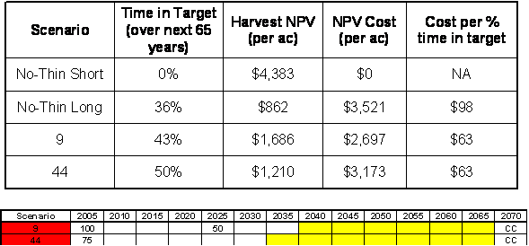
For Mid site class stands with a low starting density, the No-Thin Long scenario still takes longer to achieve the target (table 10 & 11 and figure 34) than several of the thinning scenarios. The low overstory density contributes to a dense understory. Thinning is required to reach DFC more quickly. Two thinnings provide the lowest cost but a single more aggressive thinning produces a comparable marginal cost of $63 per % time in target. With lower density the commercial alternative return is much lower so there is in effect less to lose.
| Table 10. Mid site class/low density scenarios |
 |
| Table 11. Mid site class/low density results comparison |
 |
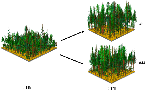 |
Figure 34. Mid site class/low density template visualization |
For High site class/low density stands (table 12 & 13 and figure 35) there is enough volume that the commercial return is high. Thinning heavy and early but only once produced the best economic return and time in target with the best marginal cost ($96 per % time in target) corresponding to the lower volume thinning which achieved the target most quickly.
| Table 12. High site class/low density scenarios |
 |
| Table 13. High site class/low density results comparison |
 |
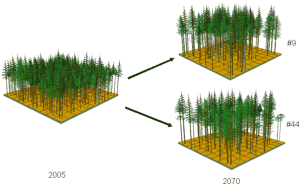 |
Figure 35. High site class/low density template visualization |
Summary of Template Pathways
Two thinning treatments rather than three generally perform best with high site stands and moderate to high density but generally resulting in higher marginal cost. High site and high density appears to be required before considering a third thinning. High site but low density is not improved with a second thinning nor is it low cost. Table 14 summarizes the best performing biopathways by site and density.
| Table 14. Summary of template pathways |
 |
With mid to high site class stands only high density stands benefit from 2 thinnings. Medium density stands provided little flexibility but all produced lower marginal cost than the higher sites with less removed and with less gained as a consequence of the low density.
Final Harvest
Time to final harvest can be extended to increase time in target but comes with an economic cost. Some stands under certain treatments may fall out of target after a period of time but most would remain in target at least for another 10 years or more. Biological legacies remaining at final harvest can improve desired conditions in subsequent rotations but are more suitable for on-the-ground management decisions than template modeling. Snags and coarse woody debris can be created on site as needed. Natural snag and coarse woody debris recruitment models are not well developed. Further the variability of snags and coarse woody debris is very large; undermining the utility of these attributes as old forest discriminators for development of management templates.
Position in target vs. time
When the test stands first reach the DFC target, they are positioned on the lower border of QMD and TPA old forest cluster as shown in figure 36. Given the variation in density the TPA ranges from a high of about 220 to a low around 100. By stand age 95, test stands have increased in QMD and decreased somewhat in TPA with most of the initially low density stands near the middle of the old forest cluster and near the owl nests (figure 36). The highest density stands have largest changes in TPA with mortality, as indicated by FVS model results, of up to 30 TPA, with less change in QMD resulting in more downed trees and snags but a slower progression into the target area than other test stands.
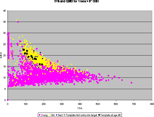 |
Figure 36. TPA and QMD for trees > 6 inches DBH |
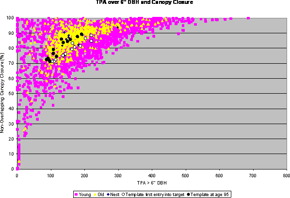 |
Figure 36. TPA and QMD for trees > 6 inches DBH |
The high density stands begin in the 80-90% canopy closure range and simply move toward the center of the cluster with tree mortality of about 25 TPA. Disturbance events such as windstorms may in fact accelerate this progression but lower the canopy closure. The less dense stands tend not to increase in canopy closure and while they move toward the center of the cluster in TPA they remain lower in canopy closure, between 70 and 80% and below many of the owl nests. Understory growth for these lower density stands is not considered by the growth model but could be expected to increase canopy density as well as TPA with both metrics narrowing the gap to the location of the owl nests.
For the very low density stands it might be argued that they are producing such poor economic returns that one strategy would be to harvest and start over making sure to get better stocking. However, these stands may be located in areas at high risk of windthrow or other conditions conducive to low density. Some of these stands will show a higher TPA as the understory matures as well as greater diameter growth of the bigger trees; in effect moving closer to the cluster center with densities moving just the opposite of the high density stands. While the comparison of the initial position of these low density stands to their terminal position may suggest they will remain low in TPA and canopy closure while at the margin of the old forest cluster, greater understory growth within these stands may increase canopy closure and TPA more rapidly than suggested by the growth model.
Step 7: Narrowing the options
If there are several viable template options, these can be further narrowed by assessment of “fine filter” performance characteristics. Outputs from LMS can be run through additional models of specific functions of interest, such as snags, LWD, etc. Adding fine filter assessments of specific functions can serve to both validate the viable options identified by the structural target approach and to discriminate or rank those options. This can help identify one or two specific options that are preferable for a template, or it can identify potential trade-offs that will need to be considered such that alternatives are included or excluded based on informed contrasts and comparisons. Since we lacked the initial data on snags and downed logs which should be valuable fine filter metrics, we have not used a supplemental fine filter for final template selection. The ratio of time in target to cost, a marginal cost for each % improvement of time in target, provides the best overall measure of performance across our treatment scenarios as it considers both the ecological metric and the cost metric. There are many cases where the highest NPV treatment alternative does not correspond to the lowest marginal cost to produce an increment of additional time in target. In most cases the highest % time in target does correspond to the lowest marginal cost.
Step 8: Creating the template
The final management trajectory diagram can be created to show the timing and target density of thinning and harvests over time for a given site class based on the chosen alternatives. It is important that a template include management flexibility, so the timing and target densities should be given as ranges rather than fixed points. For example, plus or minus 5 years on either side of a target thinning or harvest year will allow managers to have flexibility to respond to market conditions or to coordinate with other operations. Similarly, allowing a post-treatment density range of plus or minus 10-20% on either side of the target allows some operational flexibility for site-specific conditions. The resulting diagram is an easy to interpret age vs. density chart that establishes upper and lower boundaries to manage over time without additional computer modeling. While the treatments are best triggered by density thresholds, from a planning perspective they will likely first be identified by age from last treatment prior to a field inspection.
Test Stands |
Template |
|||||||||
| High Site | TPA Start |
Best thin age start |
Best thin TPA |
2nd thin age |
2nd thin TPA |
TPA Start |
1st thin age |
1st thin TPA |
2nd thin age |
2nd thin TPA |
| High-D* | 350 |
41 |
125 |
15 |
75 |
280+ |
30-40 |
110-135 |
15 |
65-85 |
| Med-D* | 220 |
34 |
100 |
15 |
50 |
200-280 |
30-40 |
90-110 |
15 |
65-85 |
| Low-D* | 170 |
31 |
100 |
15 |
NA |
<200 |
30-40 |
90-110 |
NA |
NA |
| Mid Site | ||||||||||
| High-D* | 330 |
54 |
100 |
20 |
50 |
280 |
30-40 |
90-110 |
+20 |
45-60 |
| Med-D* | 270 |
33 |
150 |
NA |
NA |
200-280 |
30-40 |
90-110 |
NA |
NA |
| Low-D* | 170 |
36 |
75 |
NA |
NA |
<200 |
30-40 |
70-90 |
NA |
NA |
*Density |
While we have created 6 possible templates to cover most of the OESF conditions, all are actually minor modifications to a basic template in order to compensate for different starting densities and site classes. As shown in table 15, most templates involve 2 thinnings but for low density situations only a first thin is applied with further density reductions expected from mortality instead of a second thin. The first treatment should be applied at age 35 with plus or minus 5 years for flexibility. As the site class gets lower one should expect the initial thinning age to increase however the OESF site class range is not large and the test stand treatment results do not suggest that a change to the initial thinning age is needed. The first thinning treatment target would generally leave between 90 to 115 trees (100 TPA) with a slightly higher leave tree target for high site and high density (110 to 135 TPA). A second thinning treatment is appropriate for high sites with medium to high density in as little as 15 years after first entry. For this treatment the leave tree target could be 50 TPA or within a range of 45-60 TPA. For medium site high density a second thinning could occur 20 to 30 years after first entry and leave about 45-60 TPA. The High site low density responded best with only one thin at 30-35 years and a leave tree target of 100 TPA (90-115 TPA range). Less trees (70-90 TPA) were left on the Mid site/low density sites. While the Mid site/medium density stand performed well retaining a higher number of trees, the initial stand condition was closer to DFC than the other test stands.
It should be noted that the first thinnings for biopathways are more aggressive than typical first commercial thins which would likely retain 150-175TPA. While heavier first thins may sacrifice maximum commercial cumulative growth potential, the resulting individual tree growth to accelerate large tree development as well as canopy openings to encourage understory reinitiation are environmentally desirable.
Step 9: Refinement and validation
Given the template performance developed for the existing test stands, timing and density targets can be modified to create additional alternatives to see if performance relative to the chosen criteria can be improved through minor adjustments. The templates can also be simulated on additional test stands to ensure that performance targets are met for a variety of starting conditions. The test stands selected for this investigation have been used to demonstrate treatment response for a range of site classes and densities representative of the majority of OESF stands. These test stands also represent the most likely age-class candidates (30-40 years) within the existing OESF inventory that might be most quickly manipulated to achieve old forest attributes. The similarity of the best alternatives confirms the potential effectiveness of biopathways for accelerating achievement of old forest conditions. Estimates of marginal costs will help to identify and refine least cost options for meeting thresholds.
Results
The templates developed cover a range of site classes and densities on the OESF. These templates can guide implementation of management strategies that achieve established environmental goals relative to the DNR HCP while helping to assure a viable economic return for trust beneficiaries. The templates are backed by a solid foundation in the literature, the use of innovative computer models, and statistically rigorous assessment procedures. This investigation builds upon previous peer-reviewed research insuring that methodologies have been tested and are robust. The templates should be easy to understand by stakeholders and policymakers, and they provide built-in flexibility that allows for site-specific discretion by forest managers. The templates also serve as a demonstration of an integrated management approach for achieving multiple objectives that can be expanded to other state forests. Development of templates for use with the Landscape Management System, software within the public domain, ensures that results are universally accessible and transparent for DNR foresters as well as other interest groups.
While prior template development research has focused more directly on Douglas-fir, these templates appear to validate that the assessment process is also effective on the generally more dense shade tolerant western hemlock stands that are common on the OESF.
While the owl nests demonstrate a tight cluster of preferences within the old forest target plots (> 80 years), the sample is sufficiently small that the templates were designed to manage for old forest habitat rather than customizing stands to owl specific preferences.
A streaming video presentation of the development and results of this project has been created for educational and training purposes. The video can be viewed online or downloaded from the Rural Technology Initiative web site:
http://www.ruraltech.org/video/2006/oesf/Default.htm#nopreload=1&autostart=1
Synergy and Future Research
This project has had the advantage of leveraging many different programs and research projects that have been developed with support from substantial public investment. Habitat suitability indices, forest structure models, carbon sequestration models, and economic assessments have already incorporated years of research from many groups and have been linked to or incorporated within LMS and tested in order to evaluate management alternatives from many different perspectives. These modeling capabilities are publicly available, resulting in applications that are robust, repeatable, and low cost. The DNR HCP has also incorporated biodiversity management pathways in their preferred Sustainable Harvest Calculation (SHC) alternative such that the assessment process will be able to advance the understanding of how best to use these pathways. This project also has the advantage of building upon an established RTI program for outreach and technology transfer to forestland managers that brings together expertise from the University of Washington, College of Forest Resources, Washington State University Extension Services and Washington Department of Natural Resources. Originally, the assessment methodology was developed to identify better alternative plans from both an ecological and economic viability perspective to reduce the motivation for small forest landowners to convert their land to other uses. It has also been used to support the development of a multi-small owner HCP for tree farmers in Lewis County. The program to compute the time in DFC was coded for easy assess by LMS to make the process for identifying time in target user-friendly and time efficient. These tools provide the ability to determine the cost to produce a wide range of ecosystem service measures that may have value in the market or through incentive mechanisms.
Future research should look at specific species habitat suitability criteria to determine how well course filter targets achieve a range of individual species needs. Fine filter parameters may prove to be useful to supplement the course filter assessment for some species. Research is needed to better understand different target conditions with the objective of improving the efficiency of providing multiple course filter objectives. Additional test stands could be examined to validate the performance for a broader range of starting conditions. Additional scenarios could be examined including efforts to determine the best pathway to restore density on minority stands where low density is a limiting factor in both ecological and economic performance. The scenarios are readily adaptable to riparian management but research could be devoted to the spatial aspects of introducing biopathways as a means of combining landscape level ecological targets on a combination of riparian and upland acres to minimize associated reductions in harvest volumes and revenues.
References
Baker, P.J., and J.S. Wilson. 2000. A quantitative technique for the identification of canopy stratification in tropical and temperate forests. Forest Ecology and Management 127:77-86.
Carey, A.B., B.R. Lippke, J. Sessions. 1999. Intentional Systems Management: Managing Forests for Biodiversity. Journal of Sustainable Forestry 9(3/4):83-125.
Carey, A.B., C.E. Eliot, B.R. Lippke, J. Sessions, C.J. Chambers, C.D. Oliver, J.F. Franklin, and M.G. Raphael. 1996. Washington Forest Landscape Management Project – A Pragmatic, Ecological Approach to Small Landscape Management. Report No. 2 USDA Forest Service, Washington State Department of Fish and Wildlife and Washington State Department of Natural Resources, Olympia, Washington. 99pp.
Commission on Old Growth Alternatives for Washington’s Forest Trust Lands. 1989. Final Report submitted to the Commissioner of Public Lands. Olympia, Washington. 40pp. plus appendices.
Crookston, N.L., & Stage, A.R. (1999). Percent canopy cover and stand structure statistics from the forest vegetation simulator. General Technical Report 24. Ft. Collins, CO: USDA Forest Service Rocky Mountain Research Station. 11pp.
DNR. 2005. Definition and Inventory of Old Growth Forests on DNR-Managed State Lands. Olympia, Washington. 21pp. plus appendices.
DNR. 1997. Final Habitat Conservation Plan. Washington State Department of Natural Resources. Olympia, Washington. 223pp. plus appendices.
DOR. 2006. http://dor.wa.gov/
Gehringer, K. R. 2006. Structure-based nonparametric target definition and assessment procedures with an application in riparian forest management. Forest Ecology and Management 223(1-3):125-138
Franklin , J.F., T.A. Spies, R. Van Pelt. 2005. Definition and Inventory of Old Growth Forests on DNR-Managed State Lands (Section One). Report to the Washington Department of Natural Resources. Olympia, Washington. 22pp.
Franklin , J.F. and T.A. Spies. 1991. Composition, Function, and Structure of Old-Growth Douglas-fir Forests in General Technical Report: Wildlife and Vegetation of Unmanaged Douglas-fir Forests. PNW-GTR-285. Pacific Northwest Research Station, USDA Forest Service.
Forsman, E.D., A.R. Giese. 1997. Nests of Northern Spotted Owls on the Olympic Peninsula, Washington. Wilson Bulletin. 109(1):28-41.
Hanson, E., D. Hays, L. Hicks, and L. Young. 1993. Spotted owl habitat in Washington, a report to the Washington Forest Practices Board, Washington Department of Natural Resources, Olympia. 116pp.
Horton, S. personal communication. DNR Olympic Region Wildlife Biologist.
Klemperer, W.D. Forest Economics and Finance. 1995. McGraw Hill. 551pp.
Lippke, B.R., J. Comnick, L. Johnson. 2004. Environmental Performance Index for the Forest. CORRIM Phase I Final Report. Module O. 13pp.
Lippke, B.R., J. Sessions, A.B. Carey. 1996. Economic Analysis of Forest Landscape Management Alternatives: Final report of the working group on the economic analysis of forest landscape management alternatives for the Washington Forest Landscape Management Project. Special Paper 21, CINTRAFOR, College of Forest Resources, Univ. of Washington, Seattle, WA. 157pp.
McCarter, J.B. 2001. Landscape management system (LMS): background, methods, and computer tools for integrating forest inventory, GIS, growth and yield, visualization and analysis for sustaining multiple forest objectives. Seattle, WA: University of Washington. 101pp. Ph.D. dissertation.
McCarter , J.B., J.S. Wilson, P.J. Baker, J.L Moffett, and C.D. Oliver. 1998. Landscape management through integration of existing tools and emerging technologies. Journal of Forestry 96:17-23.
Nigh, G. 1995. The geometric mean regression line: A method for developing site index conversion equations for species in mixed stands. Forest Science 41(1):84-98.
Oliver, C., R. Greggs, L. Hicks, S. Boyd. 1995. Forest stand structural classification system developed for the Pulm Creek Cascades Habitat Conservation Plan. Technical Report No. 10. Plum Creek Timber Company, LLP. Seattle, WA. 30pp.
Oliver, C.D. and B.C. Larson. 1990. Forest Stand Dynamics. McGraw Hill, New York. 419pp.
RTI (Rural Technology Initiative). 2001. Defining and Using Biologically Based Targets in Forest Management: Incorporating Forest Structure and Variability . RTI Fact Sheet #6. Rural Technology Initiative, College of Forest Resources, University of Washington. 4pp.
Zobrist, K.W., K.R. Gehringer, and B.R.Lippke. 2004. Templates for Sustainable Riparian Management on Family Forest Ownerships, Journal of Forestry 102(7):19-25.
Zobrist, K.W., K.R. Gehringer, and B.R.Lippke 2005a. A sustainable solution for riparian management. In Understanding Key Issues of Sustainable Wood Production in the Pacific Northwest, Deal, R.L. and S.M. White eds. USDA Forest Service General Technical Report PNW- GTR-626:54-62.
Zobrist, K. W., T.M. Hinckley, M.G. Andreu, K.R. Gehringer, C.W. Hedman, and B.R. Lippke. 2005b. Templates for Forest Sustainability on Intensively Managed Private Forests. RTI Working Paper 5. Seattle WA: Rural Technology Initiative, College of Forest Resources, University of Washington. 106pp.
APPENDIX
I. Structural Classifications (Oliver and Larson 1990)
- Old Growth (OG) = at least 6 TPA with greater than 32" DBH and at least 8 TPA that are shade tolerant (WH, RC, etc.) that are greater than 16" DBH, and at least 30% canopy closure and at least 5 snags per acre and at least 4 down logs per acre
- Understory Reinitiation (UR) = QMD of the largest 40 TPA at least 23 inches and at least a 40% canopy closure.
- Stem Exclusion (SE) = QMD of the largest 40 TPA less than 23 inches and at least a 40% canopy closure.
- Stand Initiation (SI) = QMD of the largest 40 TPA less than 23 inches and less than 40% canopy closure.
II. Structural Classifications –Carey (Lippke et al. 2004)
- Old Growth = minimum 24 inch QMD, ≥ 2 tree species, ≥ 3 conifer snags ≥ 20 inch DBH and ≥ 12 foot height, ≥ 6 logs ≥ 12 inch diameter and ≥ 20 foot length, ≥ 30% canopy closure in unmanaged forest.
- Ecologically Fully-Functional = minimum 21 inch QMD, ≥ 2 tree species, ≥ 2 conifer snags ≥ 20 inch DBH and ≥ 12 foot height, ≥ 6 logs ≥ 12 inch diameter and ≥ 20 foot length, ≥ 35% canopy closure in managed forest.
- Niche Diversification = minimum 21 inch QMD, ≥ 2 tree species, ≥ 2 conifer snags ≥ 20 inch DBH and ≥ 12 foot height, ≥ 2 logs ≥ 12 inch diameter and ≥ 20 foot length, ≥ 35% canopy closure in managed forest.
- Biologically Diverse = minimum 21 inch QMD, 1 tree species, ≥ 2 conifer snags ≥ 20 inch DBH and ≥ 12 foot height, ≥ 2 logs ≥ 12 inch diameter and ≥ 20 foot length, ≥ 35% canopy closure in unmanaged forest.
- Developed Understory = minimum 21 inch QMD, ≥ 40% canopy closure in unmanaged forest or thinned forest.
- Understory Reinitiation = minimum 16 inch QMD, ≥ 40% canopy closure in unmanaged forest or thinned forest.
- Exclusion Stage = ≥ 60% canopy closure
- Stand Initiation = all others than above to represent open structure following harvest or disturbance.
III. WAC 222-16-085 http://apps.leg.wa.gov/WAC/default.aspx?cite=222-16-085
Northern spotted owl habitats.
(1) Suitable spotted owl habitat means forest stands which meet the description of old forest habitat, sub-mature habitat or young forest marginal habitat found in (a) and (b) of this subsection. Old forest habitat is the highest quality, followed in descending order by sub-mature habitat and young forest marginal habitat.
(a) Old forest habitat means habitat that provides for all the characteristics needed by northern spotted owls for nesting, roosting, foraging, and dispersal, described as stands with:
(i) A canopy closure of 60% or more and a layered, multispecies canopy where 50% or more of the canopy closure is provided by large overstory trees (typically, there should be at least 75 trees greater than 20 inches DBH per acre, or at least 35 trees 30 inches DBH or larger per acre); and
(ii) Three or more snags or trees 20 inches DBH or larger and 16 feet or more in height per acre with various deformities such as large cavities, broken tops, dwarf mistletoe infections, and other indications of decadence; and
(iii) More than two fallen trees 20 inches DBH or greater per acre and other woody debris on the ground.(b) Sub-mature habitat and young forest marginal habitat. Sub-mature habitat provides all of the characteristics needed by northern spotted owls for roosting, foraging, and dispersal. Young forest marginal habitat provides some of the characteristics needed by northern spotted owls for roosting, foraging, and dispersal. Sub-mature habitat and young forest marginal habitat stands can be characterized based on the forest community, canopy closure, tree density and height, vertical diversity, snags and cavity trees, dead and down wood, and shrubs or mistletoe infection. They are described in the following tables:
| (i) Western Washington spotted owl sub-mature and young forest marginal habitat characteristics. |
Characteristic |
Habitat Type |
|
Sub-Mature |
Young Forest Marginal |
|
| Forest Community | conifer-dominated or conifer-hardwood (greater than or equal to 30% conifer) | conifer-dominated or conifer-hardwood (greater than or equal to 30% conifer) |
| Canopy Closure | greater than or equal to 70% canopy closure | greater than or equal to 70% canopy closure |
| 115-280 trees/acre (greater than or equal to 4 inches DBH) with | 115-280 trees/acre (greater than or equal to 4 inches DBH) with | |
| Tree Density and Height | dominants/codominants greater than or equal to 85 feet high OR |
dominants/codominants greater than or equal to 85 feet high OR |
| Vertical Diversity | dominants/codominants greater than or equal to 85 feet high with | dominants/codominants greater than or equal to 85 feet high with |
| 2 or more layers and | 2 or more layers and | |
| 25 - 50% intermediate trees | 25 - 50% intermediate trees | |
| Snags/Cavity Trees | greater than or equal to 3/acre (greater than or equal to 20 inches DBH and 16 feet in height) | greater than or equal to 2/acre (greater than or equal to 20 inches DBH and 16 feet in height) OR greater than or equal to 10% of the ground covered with 4 inch diameter or larger wood, with 25-60% shrub cover |
| Dead, Down Wood | N/A | |
| Shrubs | N/A | |
The values indicated for canopy closure and tree density may be replaced with a quadratic mean diameter of greater than 13 inches and a basal area of greater than 100.
| (ii) Eastern Washington spotted owl sub-mature and young forest marginal habitat characteristics. |
Habitat Type |
|||
Characteristic |
Sub-Mature |
Young Forest Marginal (closed canopy) |
Young Forest Marginal (open canopy) |
| Forest Community | greater than or equal to 40% fir | greater than or equal to 40% fir | greater than or equal to 40% fir |
| Tree Density and Height | 110-260 trees/acre (greater than or equal to 4 inches DBH) with | 100 - 300 trees/acre (greater than or equal to 4 inches DBH) | 100 - 300 trees/acre (greater than or equal to 4 inches DBH) |
| dominants/codominants greater than or equal to 90 feet high OR |
dominants/codominants equal to or greater than 70 feet high | dominants/codominants equal to or greater than 70 feet high | |
| Vertical Diversity | dominants/codominants greater than or equal to 90 feet high with 2 or more layers and | 2 or more layers | 2 or more layers |
| 25 - 50% intermediate trees | 25 - 50% intermediate trees | 25 - 50% intermediate trees | |
| Canopy Closure | greater than or equal to 70% canopy closure | greater than or equal to 70% canopy closure | greater than or equal to 50% canopy closure |
| Snags/Cavity Trees | greater than or equal to 3/acre (greater than or equal to 20 inches DBH 16 feet in height) OR |
N/A | 2/acre or more (greater than or equal to 20 inches DBH 16 feet in height) |
| Mistletoe | high or moderate infection | N/A | high or moderate infection |
| Dead, Down Wood | greater than or equal to 5% of the ground covered with 4 inch diameter or larger wood | N/A | N/A |
The values indicated for canopy closure and tree density may be replaced with the following:
A) For sub-mature a quadratic mean diameter of greater than 13 inches and a relative density of greater than 44;
B) For young forest marginal a quadratic mean diameter of greater than 13 inches and a relative density of greater than 28.
2) Spotted owl dispersal habitat means habitat stands that provide the characteristics needed by northern spotted owls for dispersal. Such habitat provides protection from the weather and predation, roosting opportunities, and clear space below the forest canopy for flying. Timber stands that provide for spotted owl dispersal have the following characteristics:
(a) For western Washington, timber stands 5 acres in size or larger with:
(i) 70% or more canopy cover; and
(ii) 70% or more of the stand in conifer species greater than 6 inches DBH; and
(iii) A minimum of 130 trees per acre with a DBH of at least 10 inches or a basal area of 100 square feet of 10 inch DBH or larger trees; and
(iv) A total tree density of 300 trees per acre or less; and
(v) A minimum of 20 feet between the top of the understory vegetation and the bottom of the live canopy, with the lower boles relatively clear of dead limbs.(b) For eastern Washington, timber stands 5 acres in size or larger with:
(i) 50% or more canopy closure; and
(ii) A minimum of 50 conifer trees per acre, with a DBH of 6 inches or more in even-aged stands or 4 inches or more in uneven-aged stands, and an average tree height of 65 feet or more; and
(iii) Total tree density of 200 trees per acre or less; and
(iv) A minimum of 20 feet between the top of the understory vegetation and the bottom of the live canopy, with the lower boles relatively clear of dead limbs; or
(v) Conifer stands with a quadratic mean diameter of 9 inches or more and a relative density of 33 or more or a canopy closure of 55% or more.(c) Suitable spotted owl habitat provides all of the required characteristics needed by spotted owls for dispersal.
(d) Landowners may submit information to support an alternate definition of dispersal habitat for review and approval by the department in consultation with the department of fish and wildlife.
[Statutory Authority: Chapters 76.09 and 34.05 RCW. 96-12-038, § 222-16-085, filed 5/31/96, effective 7/1/96.]
IV. Tree Species Abbreviations as they appear in Figure 21. Dominant Species
DF – Douglas-fir (Pseudotsuga menziesii)
RA – red alder (Alnus rubra
SS – Sitka spruce (Picea sitchensis)
WH – western hemlock (Tsuga heterophylla)
RC – western red cedar (Thuja plicata)
SF – Pacific silver fir (Abies amabilis)
M – indicates mixed species
| V. Detail for Figure 21. Dominant Species |
DomSpp |
Young |
Old |
Nest |
| Other | 119 |
14 |
0 |
| DF | 193 |
2 |
0 |
| MDF | 146 |
2 |
0 |
| MDFRA | 21 |
0 |
0 |
| MDFSS | 16 |
0 |
0 |
| MDFWH | 441 |
8 |
0 |
| MRA | 53 |
2 |
0 |
| MRADF | 27 |
0 |
0 |
| MRAWH | 63 |
4 |
0 |
| MRC | 5 |
13 |
0 |
| MRCWH | 16 |
27 |
1 |
| MSFWH | 17 |
12 |
0 |
| MSS | 9 |
3 |
0 |
| MSSWH | 39 |
11 |
0 |
| MWH | 425 |
137 |
3 |
| MWHDF | 482 |
21 |
0 |
| MWHDFRA | 10 |
0 |
0 |
| MWHRA | 122 |
26 |
0 |
| MWHRC | 37 |
24 |
0 |
| MWHSF | 25 |
57 |
2 |
| MWHSS | 65 |
15 |
0 |
| RA | 60 |
1 |
0 |
| WH | 434 |
279 |
3 |
VI. Detail for Figure 24. OESF by plant association |
| Unknown | Young |
Old |
Nest |
| Silver fir/depauperate | 255 |
98 |
1 |
| Silver fir/Salal/Oxalis | 133 |
32 |
0 |
| Silver fir/Alaska huckleberry | 163 |
72 |
1 |
| Silver fir/Alaska huckleberry/Oxalis | 5 |
4 |
0 |
| Silver fir/Alaska huckleberry/Queen's cup | 9 |
8 |
0 |
| Western hemlock/swordfern-oxalis | 31 |
17 |
2 |
| Western hemlock/swordfern-foamflower | 586 |
64 |
1 |
| Western hemlock/skunkcabbage | 139 |
60 |
1 |
| Western hemlock/salal | 13 |
2 |
0 |
| Western hemlock/salal/oxalis | 392 |
99 |
1 |
| Western hemlock/Oregongrape/swordfern | 78 |
22 |
0 |
| Western hemlock/devil's club | 16 |
2 |
0 |
| Sitka spruce/swordfern-oxalis | 101 |
16 |
0 |
| Sitka spruce/salal | 493 |
94 |
0 |
VII. Forest attributes reviewed as potential old forest discriminators
- Age ( ≤ 80 years; > 80 years)
- Structure classification
- Total canopy closure (%)
- Canopy closure from trees > 20 inches DBH (%)
- TPA of trees > 32 inches DBH
- TPA of shade tolerant trees > 16 inches DBH
- TPA of trees > 30 inches DBH
- TPA of trees > 24 inches DBH
- TPA of trees > 20 inches DBH
- TPA of trees > 6 inches DBH
- TPA of trees < 6 inches DBH
- QMD of largest 40 TPA (inches)
- QMD of trees > 6 inches DBH
- Average height of tallest 100 TPA (feet)
- Canopy layers (number)
- Elevation (feet above sea level)
- Dominant species
- Site index (50-year western hemlock and Douglas-fir)
- Plant association group
- Density
VIII. Treatment Alternatives
- A set of alternatives were created ranging from 0-3 thinnings with final harvest in 65 years (approx. age 100)
- Each thinning was initially done from below for all trees ≥ 6” DBH
- This not only thinned the overstory, but also removed understory trees when they exceeded 6” DBH—resulting in a “cleaning out” of lower canopy layers
- Stands fell out of the target after later thinnings
- New thresholds: First thinning ≥ 6” DBH; Second Thinning ≥ 12” DBH; Third Thinning ≥ 15” DBH
- Crown thinning
- Much better target scores
- Thinning Timing:
- 1st: Immediately for high density and some medium/low density scenarios
- 2nd: 20 (high site) or 15 years (mid site)
- 3rd: 45 years
IX. Economic Assumptions
- DOR stumpage values
- Area 1 and 2 values averaged across haul zones for quality codes 2 and 3
- Stumpage adjustments based on total harvest volume
- < 5 MBF: -$100/MBF
- 5-10 MBF: -$35/MBF
- 10-30 MBF: -$15/MBF
- >30 MBF: no adjustment
- 5% real discount rate


