Statistics For Binary
Linear Regression
The statistics were broken into steps to determine which variables
would best work for an equation. All statistics were done in SPSS.
Below are the significant steps taken and the variables in each
step. Step 3 is the most significant.
Step 1: Log10(Basize)
Step 2: Log10(Basize), Precipitation
Step 3: Log10(Basize), Precipitation, Slope
Elevation, downstream gradient and site class are not part of
the steps due to it being insignificant for the model.
| Hosmer and Lemeshow Test |
| Step |
Chi-square |
df |
Sig. |
| 1 |
8.864 |
7 |
0.263 |
| 2 |
9.9 |
8 |
0.272 |
| 3 |
10.262 |
8 |
0.247 |
| Appendix Table I1. The Hosmer-Lemeshow statistic. Indicates
a poor fit if the significance value is less than 0.05. |
Contingency Table for Hosmer and Lemeshow Test |
| |
|
Head = .00 |
Head = 1.00 |
|
| |
|
Observed |
Expected |
Observed |
Expected |
Total |
| Step 1 |
1 |
14 |
13.289 |
0 |
0.711 |
14 |
| |
2 |
10 |
9.966 |
1 |
1.034 |
11 |
| |
3 |
8 |
9.082 |
3 |
1.918 |
11 |
| |
4 |
8 |
7.142 |
3 |
3.858 |
11 |
| |
5 |
3 |
5.195 |
8 |
5.805 |
11 |
| |
6 |
4 |
3.662 |
7 |
7.338 |
11 |
| |
7 |
2 |
2.283 |
9 |
8.717 |
11 |
| |
8 |
4 |
1.572 |
7 |
9.428 |
11 |
| |
9 |
0 |
0.81 |
15 |
14.19 |
15 |
| |
|
|
|
|
|
|
| Step 2 |
1 |
11 |
10.632 |
0 |
0.368 |
11 |
| |
2 |
11 |
10.225 |
0 |
0.775 |
11 |
| |
3 |
10 |
9.602 |
1 |
1.398 |
11 |
| |
4 |
6 |
7.908 |
5 |
3.092 |
11 |
| |
5 |
6 |
5.435 |
5 |
5.565 |
11 |
| |
6 |
2 |
4.162 |
9 |
6.838 |
11 |
| |
7 |
2 |
2.679 |
9 |
8.321 |
11 |
| |
8 |
4 |
1.567 |
7 |
9.433 |
11 |
| |
9 |
1 |
0.644 |
10 |
10.356 |
11 |
| |
10 |
0 |
0.147 |
7 |
6.853 |
7 |
| |
|
|
|
|
|
|
| Step 3 |
1 |
11 |
10.903 |
0 |
0.097 |
11 |
| |
2 |
11 |
10.543 |
0 |
0.457 |
11 |
| |
3 |
11 |
9.741 |
0 |
1.259 |
11 |
| |
4 |
6 |
7.948 |
5 |
3.052 |
11 |
| |
5 |
4 |
5.371 |
7 |
5.629 |
11 |
| |
6 |
4 |
3.887 |
7 |
7.113 |
11 |
| |
7 |
2 |
2.508 |
9 |
8.492 |
11 |
| |
8 |
4 |
1.466 |
7 |
9.534 |
11 |
| |
9 |
0 |
0.554 |
11 |
10.446 |
11 |
| |
10 |
0 |
0.079 |
7 |
6.921 |
7 |
| Appendix Table I2. This
statistic is the most reliable test of model fit for SPSS
binary logistic regression, because it aggregates the observations
into groups of cases. |
|
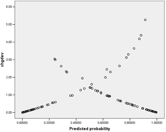
| Appendix Figure I1. Deviance
plot change helps identify cases that are poorly fit by
the model. |
|
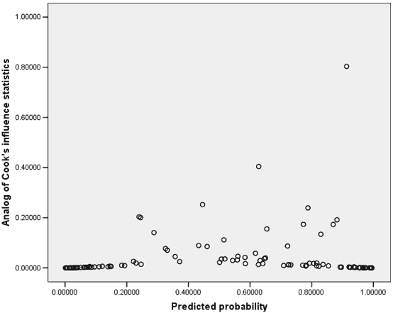
| Appendix Figure I2. The
shape of the Cook's distances plot generally follows that
of the previous figure, with some minor exceptions. These
exceptions are high-leverage points, and can be influential
to the analysis. |
Variables not in the Equation |
| |
|
|
Score |
df |
Sig. |
| Step 1 |
Variables |
PRECIP |
4.452 |
1 |
0.035 |
| |
|
Slope |
3.242 |
1 |
0.072 |
| |
|
Elevation |
2.268 |
1 |
0.132 |
| |
|
Downgrad |
0.611 |
1 |
0.434 |
| |
|
Site Class |
0.152 |
1 |
0.696 |
| |
Overall Statistics |
|
11.696 |
5 |
0.039 |
| Step 2 |
Variables |
Slope |
6.284 |
1 |
0.012 |
| |
|
Elevation |
0.45 |
1 |
0.502 |
| |
|
Downgrad |
2.153 |
1 |
0.142 |
| |
|
Site Class |
0.148 |
1 |
0.7 |
| |
Overall Statistics |
|
7.889 |
4 |
0.096 |
| Step 3 |
Variables |
Elevation |
0.644 |
1 |
0.422 |
| |
|
Downgrad |
1.126 |
1 |
0.289 |
| |
|
Site Class |
0.121 |
1 |
0.728 |
| |
Overall Statistics |
|
1.658 |
3 |
0.646 |
| Appendix Table I3. Forward
stepwise methods variables left from steps |
Model if Term Removed |
| Variable |
|
Model Log |
Change in -2 Log |
|
Sig. of the |
| |
|
Likelihood |
Likelihood |
df |
Change |
| Step 1 |
Log10(BASIZE) |
-73.474 |
55.107 |
1 |
0 |
| Step 2 |
Log10(BASIZE) |
-73.455 |
59.991 |
1 |
0 |
| |
PRECIP |
-45.92 |
4.921 |
1 |
0.027 |
| Step 3 |
Log10(BASIZE) |
-73.422 |
66.715 |
1 |
0 |
| |
PRECIP |
-44.246 |
8.363 |
1 |
0.004 |
| |
Slope |
-43.46 |
6.789 |
1 |
0.009 |
| Appendix Table
I4. The variables chosen by the forward stepwise method
all having significant changes in -2 log-likelihood. |
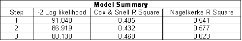 |
| Appendix Table
I5. The pseudo r-squared statistics. |
Classification Table(a) |
| |
|
|
Predicted |
| |
|
|
Head |
Percentage |
| Observed |
0 |
1 |
Correct |
| Step 1 |
Head |
0 |
41 |
12 |
77.358 |
| |
|
1 |
8 |
45 |
84.906 |
| |
Overall Percentage |
|
|
|
81.132 |
| Step 2 |
Head |
0 |
40 |
13 |
75.472 |
| |
|
1 |
9 |
44 |
83.019 |
| |
Overall Percentage |
|
|
|
79.245 |
| Step 3 |
Head |
0 |
41 |
12 |
77.358 |
| |
|
1 |
6 |
47 |
88.679 |
| |
Overall Percentage |
|
|
|
83.019 |
| Appendix Table
I6. The classification table indicating the practical results
of using the logistic regression model. |
Variables in the Equation
|
| |
|
|
|
|
|
|
|
95.0% C.I.for EXP(B)
|
| |
|
B
|
S.E.
|
Wald
|
df
|
Sig.
|
Exp(B)
|
Lower
|
Upper
|
| Step 1(a) |
Log10(BASIZE) |
5.115
|
0.935
|
29.948
|
1
|
0
|
166.464
|
26.653
|
1039.659
|
| |
Constant |
-2.711
|
0.57
|
22.617
|
1
|
0
|
0.066
|
|
|
| Step 2(b) |
Log10(BASIZE) |
5.753
|
1.064
|
29.241
|
1
|
0
|
315.028
|
39.157
|
2534.451
|
| |
PRECIP |
0.336
|
0.165
|
4.157
|
1
|
0.041
|
1.4
|
1.013
|
1.934
|
| |
Constant |
-30.754
|
13.849
|
4.931
|
1
|
0.026
|
0
|
|
|
| Step 3(c) |
Log10(BASIZE) |
7.235
|
1.425
|
25.766
|
1
|
0
|
1386.737
|
84.879
|
22656.314
|
| |
PRECIP |
0.477
|
0.184
|
6.697
|
1
|
0.01
|
1.612
|
1.123
|
2.313
|
| |
SLOPE |
0.096
|
0.04
|
5.786
|
1
|
0.016
|
1.101
|
1.018
|
1.191
|
| |
Constant |
-45.172
|
16.05
|
7.921
|
1
|
0.005
|
0
|
|
|
| Appendix Table
I7. The parameter estimates table summarizing the effect
of each predictor. |
|
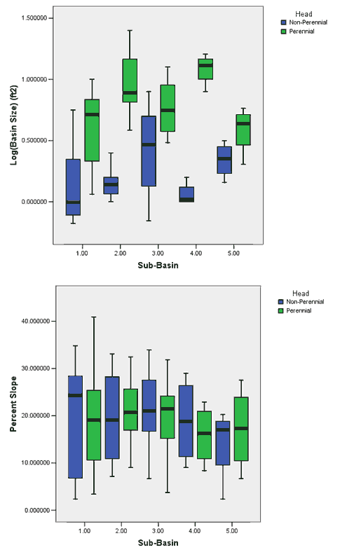
| Appendix Figure I3. Boxplots
comparing the distribution of % slope and basin size values
for PIP’s. |
|