Carbon sequestration in the Pacific Northwest: a model

A thesis submitted in partial fulfillment of the requirements for the degree of

Master of Science

University of Washington

2002

Program Authorized to Offer Degree:
College of Forest Resource

Table of Content

** Back to the RTI Theses page **

List of Figures

List of Tables

1. INTRODUCTION

Carbon dioxide is the highest emitted greenhouse gas in the world today, mostly due to fossil fuel based energy industries and deforestation (Fung 1994). The Kyoto Protocol (UNFCC 1998), the first attempt to reach global consensus on how and how much to reduce greenhouse gas emissions, described in length two key prospective solutions to the problem of balancing the carbon cycle: reduce emissions and/or sequester more carbon. The challenge is to go back to this perceived notion of equilibrium, when the quantity (mass) of greenhouse gases entering the atmosphere balances with the quantity of greenhouse gases leaving the atmosphere.

Forest and forest products have an essential role to play in the carbon cycle mitigation process because they respond directly or indirectly to the two Kyoto premises. Reducing greenhouse gas emissions can be achieved by controlling and avoiding land use changes. Deforestation in the tropics alone amounts for about 20% of total greenhouse emissions (Chomitz 2000). Using wood products that replace more energy intensive products with the same function is also part of the solution (Koch 1991). Bettering forestry related technology and management, therefore reducing energy demands for growing, harvesting and processing wood should also be considered.

On the sequestration aspect, the role of forests is essential in counteracting the carbon dioxide build up. By converting carbon dioxide to oxygen and carbohydrates through the process of photosynthesis, forest ecosystems have the ability to "sequester" carbon from the atmosphere. Carbon sink enhancement can be achieved by the afforestation of croplands and pastures, by increasing agro-forestry activities and by reforesting harvested areas (Birdsay et al 2000).

Sequestration can be defined as the net removal of carbon dioxide from the atmosphere into long lived carbon pools. These carbon pools are composed of live and dead above and below ground biomass, and wood products with long and short life and potential uses. According to the Kyoto protocol, there are three ways in which the carbon sequestered in these pools should be accounted for: afforestation, reforestation, and additionality. Afforestation implies growing trees where there were none before; reforestation addresses the idea of re-growing trees where some have been harvested, and additionality deals with the positive difference in sequestration achieved through management when compared to a base case scenario.

Generally, any approach should seek to balance emissions from forest ecosystems and the management of such, with environmental stewardship and economic growth as objectives. This is not a simple task, since it includes broad emissions inventories, emissions projections, data collection, oversight, and associated protocols. Carbon tax and carbon credit systems have been proposed to motivate increased carbon storage and/or reduce emissions (Marland et al 2001). Any system will require a credible accounting protocol to avoid counterproductive efforts. Since the Pacific Northwest is one of the most productive ecological areas of the world (Franklin & Dyrness 1973, Fujimori et al 1976, Grier & Logan 1977), and an important player in the USA forestry sector (Haynes & Weigand 1997), the creation of a carbon accounting model for the Pacific Northwest region is needed.

The carbon sequestration model is a step forward in developing a complete and interconnected set of accounting practices allowing for an accurate and credible analysis of past, present, and future carbon emissions relating to forestry in the region. The model is a tool meant to be of help in the assessment and resolution of trade offs at different levels in the management of forests in the Pacific Northwest region. It is very important to remember that although most of the sequestration and emission of carbon happens at the molecular scale, management decisions to enhance sequestration will be conducted at the stand and landscape levels. To cut or not to cut: this crucial question can only be addressed when the carbon issue is analyzed on a broader spectrum. The model incorporates accounting from the standing forest to the product level, wood-steel substitution dynamics in construction and biofuel displacement of fossil fuels, together with emissions from the forest operations and manufacturing activities.

Issues such as increasing the stock of carbon in the existing forests (additionality), together with more efficient harvest techniques and greater usage of wood in long lasting products (such as steel substitution in construction), and the displacement of fossil fuels by biofuels should be considered when addressing the carbon question and its possible trade offs in time and space.

Can forests be managed to meet the multiple goals of providing habitat, wood products, economic returns and carbon sequestration? The carbon model is one more tool available to managers to help in the attempt and realization of this goal.

2. LITERATURE REVIEW

It has been widely acknowledged that global anthropogenic emissions of carbon dioxide and other greenhouse gases may seriously affect the global climate system. The disruption of this cycle can have significant consequences on life as we know it (Hansen, 1988; Schneider, 1989; IPCC 1992). In 1996, 150 countries signed the United Nations Framework Convention on Climate Change (Anonymous 1992), with the objective of achieving the "stabilization of greenhouse gas concentrations in the atmosphere at a level that would prevent dangerous anthropogenic interference with the climate system". Much effort is currently focused on ways of reducing carbon dioxide contributions to the atmosphere going from researching the science to understanding the fundamental biological and ecological processes in unmanaged and managed terrestrial ecosystems, to the development of protocols and new policies to address this global environmental dilemma. Carbon dioxide is one of the greenhouse gases that cause the earth's atmosphere to warm up, allowing the short-wave length solar radiation to come in, but trapping much of the long wave out going radiation. This interaction is a major determinant of global temperatures and many scientists believe that the average global temperature has risen by .5 to 1oC in the last century (IPCC 1992). Today's atmosphere contains about 370 parts per million CO2, as compared to about 280 ppm before the industrial revolution, and levels are increasing at about 0.5 % per year (Brady 1996).

Carbon is the foundation of life. All living tissues have carbon atoms in their composition and the cycle of this element is basically the cycle of life in our planet. The carbon cycle involves the soil and all vegetation and animal life on earth. Plants absorb carbon dioxide from the atmosphere and through photosynthesis, capture the carbon molecules for energy and build up of structural components. Part of this carbon returns to the atmosphere soon after being processed through respiration. Other parts stay as standing biomass for some time, returning to the cycle as organisms die and decompose. Some of the standing biomass will eventually be eaten by animals, with half of it exhaled immediately, the other returned as bodily wastes to the soil later in time. Once in the soil, microorganisms metabolized them, gradually returning them to the atmosphere, or leaching out as carbonates through the soil (Figure 1).

Figure 1. The carbon cycle on Earth. Illustration from NASA Earth Science Enterprise

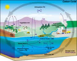
Understanding the factors and processes driving and influencing the cycle of carbon in a particular ecosystem is critical to achieve proper management of the aboveground biomass and soil organic matter, whether it is for reducing greenhouse gas emissions or improving soil quality.

2.1. Forest Ecosystems

Forest ecosystems have essentially three carbon pools: the living biomass, detritus (debris from dead plants and animals) and soils. Soils contain almost twice as much carbon as the aboveground vegetation and the atmosphere carbon combined (Brady 1996). Through the decomposition and the accumulation of organic matter, soils have a major effect on the regulation of the carbon cycle. When soil and aboveground organic matter decline, atmospheric carbon increases, with global consequences, such as the greenhouse effect. Potential mechanisms for reducing net carbon emissions through increased carbon sequestration include the forest ecosystem together with the forest socio-economic system, with both of those systems dynamic's affecting the carbon cycle. Conservation and adaptive management of existing forests, the establishment of new forests (forest ecosystem level) and the substitution of fossil fuel based energy and products by wood biomass (forest socio-economic system) could further increase the fixation of carbon from the atmosphere (Kohlmaier et al 1998).

Forests store carbon as they accumulate biomass, but forests are also commercial sources of timber and wood fiber. In most carbon accounting budgets, forest harvesting is usually considered to cause a net release of carbon from the terrestrial biosphere to the atmosphere (Houghton et al 1983, Harmon et al 1990). As the debate about controlling or mitigating atmospheric carbon dioxide concentrations moves from the study of the scientific issues to a search for practical solutions, a central question becomes whether commercial use of forests could be managed to contribute to terrestrial sequestration of carbon. Can forest management practices be developed so that they meet the multiple goals of providing wood and paper products, economic returns from natural resources, and also sequester carbon from the atmosphere?

In managed forests, the amount of additional carbon sequestered will be determined by three factors: the increase of standing carbon biomass due to land use changes and increased productivity, the amount of carbon remaining below ground at end of rotation, and the amount of carbon sequestered in products and energy, including their disposal (Johnsen et. al. 2001).

As stated previously, forests represent a huge storage of carbon since they hold about 80 % of the carbon fixed in the living biota, and much interest and effort has been put into their study, because of the possibility of being directly altered by human activity (Apps & Price 1996). The role of forests, as sink and sources of carbon in the carbon cycle, is not static at any spatial or temporal scale. Temporal changes in the forest ecosystem carbon pools are mainly driven by the dynamics of the carbon pools. Keeping track of the ecosystem processes, including population dynamics, is a crucial part of the carbon assessment. This assessment should be done at the stand level, which is believed to be the appropriate scale for such analysis (Apps & Price 1996; Harmon 2001). Forest ecosystems are complex, dynamic and diverse. Forest stands can be complex, dynamic and diverse. They all have however, three carbon pools: the living biomass, detritus and soil pools. All of these components have a role in the carbon cycle dynamics. The soil, a natural body of organic and inorganic materials and living forms, provide the substrate for plant growth. Detritus, the debris from dead plants and animals, is a source of storage as well as a source of food. The live biomass, which includes above and below ground pools, composed of coarse and fine roots, understory and canopy, captures carbon dioxide while releasing oxygen, and also respires, releasing part of the carbon dioxide previously absorbed.

A more detailed literature review will be given first for soil, followed by above and below live biomass. Lastly, the detritus component will be explored, including plant debris (litter fall) and harvest residuals (slash).

2.1.1 Soils

Conversion of natural to agricultural ecosystems has lead to drastic perturbations in the processes governing the soil organic carbon dynamics. Deforestation, biomass burning, plowing, residue removal, fertilization and single crop cycles have been depleting the earth's soils in most agroecosystems by 50 to 70% (Lal 1995). The effects of forest management on carbon soil storage are not as clear nor as well understood as in agricultural systems. Estimated carbon storage in below-ground components is known and has been measured (Brady 1996), but it is mostly how harvesting and management affects the soil carbon where knowledge is lacking.

Soil carbon has been found to be strongly dependent on the stand composition and climate (Schlesinger 1977), therefore very hard to model. Organic carbon in the root zone accounts for approximately 2/3 of the carbon in terrestrial ecosystems worldwide (Post et al. 1982). It is less responsive to harvest than the litter fraction because of its long residence time. Turn over rates encompass a large range. Post et al (1982) estimated a turn over rate of 0.00083 per year, although faster turn over rates have also been shown: 0.013 per year (Gardner & Mankin 1981) and 0.025 per year (Schlesinger 1977).

Harvesting can have a significant increase or decrease effect on forest floor biomass, mostly based on how much slash is left behind after the operation (Johnson 1992). The majority of studies however, showed little or no change in the soil mineral carbon after harvest, with less than 10 % increase or decrease (Fernandez et al., 1989; Johnson et al., 1991; Aztet et al, 1989, Huntington and Ryan, 1990; Alba and Perla, 1990; Lawson and Taylor, 1990; Raich 1983). Exceptions are usually found after harvesting in tropical areas, where soils are poor and the environmental condition are proper for rapid decomposition. Houghton et al (1983) developed a global carbon model, in which the assumption is that after forest harvest, tropical, temperate and boreal ecosystems loose 35, 50 and 15 % of litter and soil carbon. Harmon et al (1990) assume no change in soil carbon although noted that most probably soil organic matter would decrease with intensive forest management.

Fire, be it a prescribed or a wild fire, will reduce the carbon and the overall floor biomass, the effects depending primarily on the intensity of the burning, with the upper 15 cm., the surface soil, most readily influenced by land use and soil management. In the Pacific Northwest, a study found significant losses of floor biomass and nitrogen (40%) after a wildfire (Grier 1975). Another study, this time on broadcast burning, found a decrease in soil carbon (20-30%), with an equal or higher increase in the soil carbon almost two years after the prescription (40-70%) (Macadam 1987).

Carbon soil can be increased with fertilization, because of its effect on primary productivity. Effects of nitrogen fixation and fertilization on soil carbon have given results on carbon soil increasing from 30 to 100 % depending on the site and the species mix composition (Alnus rubra and Ceanothus spp.) (Binkley 1983; Binkley et. al. 1982). Despite all the unknowns and uncertainties of soil carbon dynamics and management impact on those dynamics, the commonly held assumption of soil carbon losses of 30-40% (Musselman and Fox 1991) after harvesting was not corroborated by the literature review.

2.1.2 Above ground living biomass

Different studies present a dichotomy on aboveground biomass dynamics, with some suggesting aboveground components can be a net sink (Delcourt & Harris 1980, Oliver et. al. 1990) or a net source (Houghton et. al. 1983; Harmon et. al. 1990) of carbon. Both cases are correct. The analysis and assertions on what an ecosystem's carbon is or will become under a certain line of management will depend on what was the state of the ecosystem before any management was conceived. Furthermore, it will depend on how extensive is the spectrum under which carbon cycling is considered. For example, Harmon et al (1990) argued that the conversion of old-growth forests to younger forests under current harvesting and use conditions has added and will continue to add carbon to the atmosphere, even when considering long term products such as lumber. Oliver et al (1990) found similar results at the forest ecosystem level, but further argued the conversion of old growth to managed stands is negligible when compared to the addition of carbon by the burning of fossil fuels. Similar results were found by Schlamadinger and Marland (1996). This is why it is very important to establish first and foremost the spectrum under which the carbon accounting story will be evaluated. Nobody would deny that an old growth stand stores more carbon at the forest level than a younger stand, and that the younger stand has a greater primary productivity, with higher rates of yearly uptakes of carbon. With these differences taken into consideration, the above ground living biomass is further analyzed.

In the development of a forest, the foliage, litter fall, net primary production and nutrient accumulation in above ground tree components usually reach a plateau at the stem exclusion stage (Tadaki 1966, Gessel & Turner 1976, Oliver 1981, Sprugel 1985). This trend seems to be true for Douglas-fir as well (Turner & Long 1975) and directly impacts the development of biomass through time in the different components.

The distribution of standing forest biomass in representative stands in the Pacific Northwest region has been previously estimated (Grier & Logan 1977, Keyes 1979, Edmonds 1980, Vogt et al 1980, Gholtz 1982, Cooper 1983, Keyes & Grier 1981, Santantonio & Herman 1985, Vogt et al 1986, Edmonds 1987). The total biomass and forest carbon will depend on the stand conditions, its age, density, species composition, etc. However, the patterns of biomass distribution in conifer stands of the forests of the Pacific Northwest are very similar and roughly as follows: 65-75% in the stem and bark, 15-20 % in coarse roots, 5-10 % in the crown (branches and foliage). Biomass in stem and bark on a 40 year old Douglas fir stand on a high productivity site was about 76 % (Cooper 1983), and this proportion was about 73 % in a low productivity site planted with Douglas-fir (Keyes & Grier 1981). Similar values have been established for old growth Douglas-fir in western Oregon (Grier and Logan 1977).

Looking at the components on conifer stands separately, a nearly complete foliage cover is established early in stand development of most forests and remains essentially constant until maturity (Grier & Logan 1977, Keyes 1979, Cooper 1983). Branches, as extensions of the stem, can accumulate carbon through the life of the tree. The fraction of biomass in branches is usually higher for hardwood stands, with as much as 25 % of the biomass found in that component. This proportion is much smaller for conifer trees, with about 5-7 %. The stem biomass increases rapidly with age while the foliage biomass stays fairly constant (Grier and Logan 1977).

Carbon content is approximately 50 % of the oven dry weight (Reichle et al 1973, Harmon et al 1990) with slight differences related to the chemical and physical composition of some of the components (Vogt 1991).

2.1.3 Below ground living biomass

The importance of roots as structural, storage and physiological organs has been acknowledged for quite some time (Harris 1971, Santantonio 1977). However, they have not been, for the most part, included in ecosystem research because of the difficulties surrounding their study. Observations are not possible without major disturbances in the soil, while changing dramatically the environment of the roots.

The development and buildup of the roots biomass is more complex than some of the above ground components. This is due to the variety of roles played by coarse and fine roots: structural support, food storage and nutrient absorption for example. However, in their 1992 study on spatial disposition and extension of the structural coarse root system of Douglas-fir, Kuiper & Coutts found significant positive correlations between all the coarse root parameters studied and the tree diameter at breast height (dbh). Furthermore, data on the relationship between coarse root biomass and dbh in Douglas-fir in the Netherlands was found to be consistent with natural stands of Douglas-fir in the Pacific Northwest (Santantonio et al. 1977), even though the site conditions and management history between the two sites were very different. Dbh, which is readily available, has therefore been shown to provide good estimates for woody root biomass.

Decomposition rates for woody roots in forest ecosystems of the Pacific Northwest were estimated by Chen et al. (2001), with Douglas-fir roots having an estimated decomposition rate of 0.05/year for roots between 4 and 12 cm.

Fine roots on the other hand are very hard to account and simulate based on growth models. An extensive study on fine root biomass related to stand age and productivity found no significant differences among stands of different age but same site productivity (Vogt et al 1987). Another study did a sensitivity analysis dealing with the incorporation of fine roots biomass into the soil carbon, leading to the assumption of fine roots flux being relatively constant (Cropper and Ewel 1984). In biomass studies and budget estimations, fine roots biomass estimates from previous studies are added to the total estimated by the simulations (Harmon et al 1990, Keyes & Grier 1981), or total root biomass is based on a percentage of the bole (Bruschel 1993), but none of the studies from the literature reviewed provided a potential way of simulating their growth and death.

2.1.4 Forest floor

2.1.4.1. Plant debris

Carbon accumulation in detritus and soil often accounted for greater quantities of biomass than the living biomass, especially on hardwood stands (Schlesinger 1977, Covington 1981, Gholz & Fisher 1982, Moore & Braswell 1994). The return of organic litter to the forest floor is complex and very variable. Factors to consider among others are: the age of the stand, the species composition, the density of stand, the site productivity and the environmental conditions (Bray & Gorham 1964). It is clear that litter-fall plays a fundamental role in soil formation and site productivity (Bray & Gorham 1964, Schlesinger 1977, Covington 1981, Gholz & Fisher 1982, Moore & Braswell 1994). It is also clear that both the carbon chemistry and nutrient concentrations of litter strongly affect its decomposition (Aber et. al. 1990). Thus, detrital mass changes more rapidly than soil carbon with disturbances.

2.1.4.2. Logging debris: slash

Slash burns are very rarely done anymore and have not been done for most of the last 20 years because of smoke. On the west side of Washington Cascades, on slide ground, the slash is left unburned unless whole tree yarding is the harvest method. In the case of whole tree yarding, logs are processed by a delimber and slash is burned on the landing. On gentler terrain, where the cut-to-length system is used for thinning, slash remains unburned. When shovel logging is the harvest technique for a clearcut, burn piles are created and combustion is fairly complete (Mason, personal interview, 11.2001).

Harvesting can have a significant increase or decrease effect on forest floor biomass, mostly based on how much slash is left behind after the operation (Johnson 1992).

2.2 Managing for carbon sequestration: the Silviculture

2.2.1 Longer rotations

Long rotations develop structurally complex managed forests and increase the accumulated timber volume per unit area (Franklin et al 1997, Burschel et al 1993). Longer rotations are ecologically viable because Douglas-fir (Pseudotsuga heterophylla) and other associated conifers can live to a very old age and their productivity is maintained to advanced ages (Curtis 1997). Longer rotations should be combined with thinning regimes to increase the productivity and the size of trees in a shorter time span. Larger trees imply higher wood quality, and the thinning regimes can provide revenue as intermediate operations. Longer rotations allow for adjusting unbalanced age distributions, increasing the quality of wildlife habitat associated with late successional forests, and increasing the net standing carbon storage capacity.

2.2.2 Variable retention

The variable retention system (Franklin et al 1997) is based on the concept of retaining structural components of a particular stand for at least another rotation. The development and maintenance of a structurally complex forest is the most important point when talking about the restoration of a forest. It is very flexible and the level of retention directly relates to the management objectives. It is important to consider other functions of these structural components, beyond the carbon sequestration per se, such as the enriching attributes and enhancement of connectivity throughout the landscape. The idea is to provide structural elements for diverse habitat requirements, ameliorate the microclimatic conditions, and maintain microfauna (mycorrhizal fungi, lichens etc). Enriching stand structure by maintaining living and dead structural material of various sizes, species, and levels of decay through aggregated or dispersed retention can also be incorporated into the management of the forest. Leaving behind coarse-woody debris following thinning and harvesting operations is recommended to increase the carbon in the forest floor.

The management objectives will determine what will be retained, how much and in what pattern. Large trees with special features such as rot pockets, cavities and large limbs or clusters of limbs should be retained. Snags in different states of decay and sizes, as well as coarse woody debris in different sizes and stages of decay should also be retained. The pattern in which these structures are to be left will depend on the stand and its characteristics. Aggregated retention will be preferred at some points, and dispersed retention will be the choice on others, hopefully through the mixture achieving greater complexity and carbon sequestration. Shelterwood (Smith et al 1996) for example, is a type of dispersed retention of dominant and co dominant wind firm and stress tolerant trees, that will provide in time a well distributed source of snags and coarse woody debris.

2.2.3. Thinning regimes

Thinning can be used to promote the overall health of a forest, through reduction of high fuel loads and increased wind stability. Thinning can be used to salvage material from disturbances and avoid insect outbreaks (Smith et al 1996, Oliver & Larson 1996). This is an important consideration when addressing issues such as fire safety, insects, wind stability and diseases. More important however, thinning can be used to accelerate the stand dynamics of a particular stand, favoring certain structural components that have a functional value, releasing growing space for understory species and advanced regeneration, or simply to increase the size of trees. Thinning in restoration is used as a tool that affects the structure of the stand. Pre-commercial thinning (PCT) is applied near the end of the stand initiation to enhance survival, growth and value of the residual trees. It increases stand uniformity but promotes tree growth and understory development (shrub and herbaceous) allowing also for early establishment of shade tolerant species (Oliver and Larson 1996). By doing a PCT, the differentiation of the stand is accelerated and the structural and species components increased. The spacing can vary in patches through the plantation, with small openings or gaps created to retain components of the early initial stage.

Thinning combined with extended rotations can maintain forest cover for long periods while still providing wood products, through allowable intermediate operations; timber flow can be sustained during intermediate stages of development with the benefit of ecological processes being maintained and higher wood quality achieved (Oliver 1993, Burschel et al 1993).

2.3 Accounting for the sequestered carbon

The Kyoto Protocol to the United Nations Framework Convention on Climate Change (1998) prescribes that net flows into or out of the biosphere will be represented by the changes in carbon stocks. This notion simplifies the measurements and accounting processes. The Intergovernmental Panel on Climate Change (2000) is consistent with this prescription, defining carbon sequestration as an increase in carbon stocks anywhere but in the atmosphere. The important issue is "additionality" (Chomitz 2000). Additionality addresses the idea that carbon sequestration or reduced emissions can result from a management change. Management alternatives can be compared against a base line, to measure the change from "business as usual". Afforestation of grazing land for example, is a one time huge addition of carbon pools and if reforested after disturbance, the carbon pools can be maintained through a long period of time.
How do we measure carbon and how can we estimate the variations in the different terrestrial pools? Biomass is one of the key characteristics of forest ecosystems because it contributes in the definition of carbon flux and nutrients, as well as the potential standing and dead organic matter in a particular site. Biomass studies are essential for understanding ecosystem dynamics. Biomass studies are static however, describing and estimating living and dead material in a particular stand at a particular time (Santantonio et al 1977). Combining biomass studies with growth models seems to be the most straightforward manner for estimating component masses at different points in time at the stand scale. The carbon storage pattern simulated by the model is static, meaning productivity of site is assumed constant as embedded in the original inventory in question, without possible changes associated to different temporal scales, like the global warming issue. The Kyoto Protocol specifies integration of greenhouse emissions with corresponding offsets credits if carbon is removed from the atmosphere on a 5-year commitment period. Integration over spatial scale might be used as well to decrease the costs in accounting, monitoring and verification.

2.4 Forest products, biofuel and substitution

Harvesting of forest ecosystems changes the natural carbon cycle between the terrestrial pools and the atmosphere. Therefore, the balance between forests and forest products is an important component in any budget analysis and should be included.

The carbon fluxes related to the harvesting activities should follow the general equation for atmospheric flow (Winjum et al 1998): net carbon flux to the atmosphere = carbon fluxes to the atmosphere from harvesting activities and forest products - carbon sequestration during development of the forest. The carbon fluxes associated with forest harvesting activities and the use of wood should include the carbon emissions from decomposition of slash left in the forest after harvest, the burning of fuelwood, the waste from manufacturing wood products, and the decay of the products pool.

Over a long term period, the amount of carbon stored in the biosphere reaches a steady state, and continuing mitigation of carbon emissions depends on the degree fossil fuel use is displaced by biofuel and wood products (Schlamadinger & Marland 1996).

2.5 Carbon credits

The Kyoto Protocol to the United Nations Framework Convention on Climate Change (1998) has proposed a way for establishing limits on greenhouse gas emissions to be enforced internationally, with different types of commitments for developed and developing countries. The protocol allows, within a set of rules, for countries to use their terrestrial sinks to offset part of their greenhouse gas emissions from other sources.

The idea of emission trading has also been included in the Kyoto protocol. Countries listed in Annex B of the protocol can offset their own emission reduction commitments by engaging in emission reduction activities in another Annex B country (developed) or a non Annex B country (developing). The protocol is however unclear if carbon sequestration can be used the same way the emission reductions activities are carried between Annex and non Annex B countries. Among other issues to be resolved before the Kyoto protocol can be implemented internationally and commitments enforced internationally, is that accounting rules for emissions and reductions need to be tested and put in place (Marland et al 2001).

3. METHODS

3.1 The Forest carbon

The carbon forest module includes the following components: branches (dead and live), foliage, stem and bark, standing dead trees (snags), coarse roots and litter (harvest slash, dead branches and foliage). Forests are considered a standing pool of carbon at any point in time.

The forest module of the carbon model is based on accounting for all allocations through biomass estimates at discrete points in time, which establishes where and how much is sequestered in what components. This allocation changes in time through losses by decomposition, and harvest operations that use fossil fuels.

Carbon additions or reductions to atmospheric pools resulted from forest growth, silvicultural treatments and decomposition. These additions (sequestration) and reductions (emissions) were calculated as the difference between total estimated forest carbon storage the growth period before treatment and total estimated forest carbon storage for the growth period post treatment (Figure 2).

Figure 2. Forest module based on carbon sequestration (additions) and carbon emissions (reductions).

Soil carbon changes were ignored due to the complexity of assessing carbon budgets through time after silvicultural operations, and from the leaching of organic and inorganic carbon at that level (Harmon et. al. 1990). Research attention has been given to below ground processes, respiration and foliage dynamics (Landsberg et. al. 1991), and as information becomes pertinent should be integrated to the system.

The model has been developed for 5 year growth periods, but LMS allows for an increase of this time for operations assessed with 10-year growth periods, in which case equations would account for this change.

The first step is to convert the LMS scenario tables for the forest, the cut and the snag inventory from English to metric units to be consistent with the units required for the regression equations used. The scenario table shows individual tree records with its respective attributes for all the management periods considered. Regression equations developed by Ghotlz et al (1979) were used to estimate tree component dry weight biomass based on diameter at breast height (d.b.h.) for branches, foliage, stem, bark, snags and coarse roots in kg/ ha. High correlations are usually found in logarithmic regressions of dry weight on d.b.h. According to Bunce (1968), this is in part due to the balance between apical and radial growth, and because logarithmic units represent progressive orders of magnitude. The estimation of current and total foliage biomass using d.b.h. has been shown to have errors in the regression, especially in older stands, and this should be taken into account (Grier & Waring 1974, Snell & Brown 1978, Marshall & Waring 1986). All results however, are benchmarked against biomass estimates found in the literature (Grier & Logan 1977, Keyes 1979, Edmonds 1980, Vogt et. al. 1980, Gholtz 1982, Cooper 1983, Keyes & Grier 1981, Santantonio & Herman 1985, Vogt et. al. 1986, Edmonds 1987, Vogt 1991). The equations, unless cited otherwise, follow the form:

(1) ln Y = a + b ln X,

where a and b are regression coefficients, Y is the dependent variable and X is the independent one. The equations are species and component specific and have been used in several biomass studies in the region to determine dry matter production (Grier and Logan 1977, Gholz 1982, Cropper and Ewel 1984, Vogt et al 1987, Harmon et al 1990, Canary et al 1996). Derived from equation (1), the equations for biomass (B) follow one of the three forms, depending upon species and component (Appendix A):

(2) B = e ^b0 * dbh ^b1

(3) B = b₀ + b₁ * dbh ² * ht/100 - b₂ * (dbh ² * ht/100) ²

(4) B = b₀ + b₁ * (dbh ² * ht/100)

where b₀, b₁ and b₂ are regression coefficients that are species and component specific (Ghotlz et al. 1979). Standing carbon was estimated by multiplying the biomass output by a proportion factor that depends on the species and component, but averages 50% of dry weight (Reichle et al 1973, Harmon et al 1990, Birdsay 1992). The carbon output is then summarized into three groups: stem (bark and trunk), crown (foliage and branches) and soil (coarse roots). The understory carbon pool represents approximately 1% of forest carbon (Turner at al 1995). Since this is a small percentage of the total forest carbon pool and because models are not available to link understory biomass to tree inventories, estimations of understory carbon storage were not included in this project.

(5) SB = (biomass of live tree stem (Gholtz et. al. 1979) * density of snag (Spies
1988)) / density of live tree (Hartman et al. 1976)

The snag carbon content was estimated by multiplying the snag biomass times the species carbon factor, which is very close to the live tree carbon factor. The change in carbon content with regards to the biomass of the component remains relatively constant between live and dead trees (Sollins et al 1987). Existing stumps were not considered in the carbon pool, because data on those components was not available for calculation.

The reduction of the different biomass pools, such as snags, litter fall and coarse roots were estimated by decomposing them according to species specific annual decomposition rates developed by Harmon (1993)(Appendix A) based on the literature (Harmon et. al. 1986). They have been evaluated and used by major studies (Turner et al 1995, Birdsay 1996). Estimation of subsequent reductions of carbon from the decomposing components from the forest module were calculated using the following equation:

(6) X_t = X₀ (1- k * t ) ,

where X_t is the carbon biomass at time t, X₀ is the initial biomass, k is the species specific constant describing the biomass loss per year and t is time in years (Aber and Melillo 1991). The mass of decomposing material is the sum of mortality in the most recent interval (5 year periods) and the residual mass of decomposing material (X_t).

Because LMS projections work on 5 year steps, the equation generally used within the model follows the form:

Total Xt₁ = Xt _0->1 + ((1-k)⁵ * Xt₀),

where Total Xt₁ is the cumulative carbon in a certain component at time t₁, Xt _0->1 is the carbon accumulated in that component in the period t₀ to t₁, k is the decomposition rate, 5 is the number of years and Xt₀ is the carbon found in that component at time t₀.

3.2 The Carbon in Products

Carbon sequestration goes beyond what can be measured in the forest as live and standing or dead and decomposing. Forest products constitute a very important pool for capturing carbon on a long-term basis, especially when emphasizing the use of wood on long term products, such as lumber for structural components in residential construction.

Products are modeled with a constant rate of products loss to the atmosphere, as most studies that have addressed products have done (Houghton et al. 1983, Harmon et al 1990, Oliver at al 1990, Dewar 1991, Harmon et al. 1996). The model does not allow for changes in time in terms of technological improvements in manufacturing efficiencies and product use, and does not include disposal since it includes continuous decomposition. The model considers the raw biomass harvested, its conversion to products through manufacturing, and the accumulation and decomposition of the product pool through time.

The products module takes all the biomass harvested at different points in time, allocating part of it to long term and part to short term carbon pools. The long term products constitute the base for the substitution assessment. The short term products are the base for the displacement of fossil fuels by biofuels. Harvesting and manufacturing emissions are also part of the carbon model accounting (Figure 3).

Figure 3. The products module and its components within the carbon model.

Starting with the Volume summary table from LMS, with forest and cut volumes for a particular scenario, the amount of forest products is determined by using a set of studies recently conducted in the Pacific Northwest by C.O.R.R.I.M. (2002). Four mills were surveyed in the region, producing dimension lumber as their primary output. The manufacturing process was divided in four units: sawing, drying, planing and energy generation. The numbers, coefficients and factors used in this part of the carbon model are the average values derived by weighting the production at each one of these mills (Appendix B).

The spreadsheet starts with total raw volumes of harvested material per stand given in ft³/acre. Using an average lumber yield of 9.9 bf/ ft³, volumes in ft³ are converted to Mbf (thousand board feet) of dry planed lumber. In order to produce one Mbf of dry planed lumber, 101.01 ft³ of raw logs are required. This standard yield is neither species nor diameter sensitive. The four mills reported a range from 90.4 to 105 ft³ of logs /Mbf of lumber. A wood density of 28.08 lbs/ft³ was used for Douglas-fir and 26.21-lbs/ ft³ for western hemlock (US Forest Products Laboratory, 1999) to convert volumes to mass.