|
Here's a link to the PDF version
of this Thesis
By
Kevin R. Ceder
A thesis submitted in partial fulfillment of the
requirements for the degree of
Master of Science
University of Washington
2001
Program Authorized to Offer Degree: College of Forest Resources
TABLE OF CONTENTS
List of Figures
List of Tables
Introduction and Objectives
Background
Original Habitat Evaluation Procedure
Other Approaches To Habitat Evaluation
Proposed Pathways
The Landscape Management System
Methods
Study Area
Field Procedures
Lab Procedures
Data Analysis
Results
Validation
Landscape Simulations
Pathway Simulations
Discussion and Management Applications
Habitat Model Responses
Management Applications
Advantages Of Integrating HEP and LMS
Limitations Of Integrating HEP and LMS
Conclusion
Bibliography
Appendix A: Tabular results
from Landscape Management Simulations (PDF
Here)
Appendix B: Satsophsi.py
documentation and computer code (PDF
Here)
Satsophsi.py Program File Documentation
Satsophsi.py Computer Code
Appendix C: Hsi.ini Configuration
File and Documentation (PDF
Here)
Hsi.ini Configuration File Documentation
Hsi.ini Configuration File
List of Figures
| 3.1 |
Location map of Satsop Forest in Southwest Washington |
| 3.2 |
Orthophotograph of Satsop Forest with stand boundaries |
| 3.3 |
Map of Satsop Forest cover types |
| 3.4 |
Map of Site Classes on Satsop Forest |
| 3.5 |
Map of age classes on Satsop Forest |
| 3.6 |
Map of species distribution on Satsop Forest |
| 4.1 |
Mean difference between HSI values reported in
original HEP and values calculated by LMS using original HEP
data, with 95% confidence intervals |
| 4.2 |
Mean difference between HSI values reported in
original HEP and values calculated by LMS using 1998 Satsop
Forest inventory data, with 95% confidence intervals |
| 4.3 |
Habitat flows for landscape simulations |
| 4.3 (cont.) |
Habitat flows for landscape simulations |
| 4.4 |
Harvested volumes by size class for five-year
projection periods |
| 4.4 (cont.) |
Harvested volumes by size class for five-year
projection periods |
List of Tables
| 2.1 |
Timbered cover type thresholds for Satsop Forest
from the original HEP |
| 3.1 |
Cover type acreages and number of polygons |
| 3.2 |
Site Class to 50-yr Site Index |
| 4.1 |
Habitat units for all species modeled for 1998,
2038 and 2078 |
| 4.2 |
Annual average harvested volumes (mbf/yr) and
percentage in each size class from landscape simulations |
| 4.3 |
HSI values and top five pathways for individual
pathway simulations using young dense stand |
| 4.4 |
HSI values and top five pathways for individual
pathway simulations using young open stand |
| 4.5 |
HSI values and top five pathways for individual
pathway simulations using old single storied stand |
| 4.6 |
HSI values and top five pathways for individual
pathway simulations using old multiple storied stand |
| 4.7 |
Total harvested volumes (mbf/ac) and top five
pathways for individual pathway simulations using young-open,
young-dense, old-single-story, and old-multiple-story stands |
| 5.1 |
Comparison of annual harvested volumes (mbf/yr)
to percent changes in wildlife habitat over an 80-year simulation
|
| 5.2 |
Twenty pathways with highest average HSI values
over an 80 year simulation for stands initially 10-years old,
open (~435 tpa) and dense (~1300 tpa), with species benefited |
| 5.3 |
Sixteen pathways with highest average HSI values
over an 80 year simulation for stands initially 90-years old,
single and multiple layered canopy, with species benefited |
| 5.4 |
Total harvested volume (mbf/ac) from an initially
10-year old stand during an 80-year simulation for 16 top habitat-producing
pathways and species benefited |
| 5.5 |
Total harvested volume (mbf/ac) from an initially
90-year old stand during an 80-year simulation for the 16 top
habitat-producing pathways and the species benefited |

Introduction and Objectives
The public has become increasingly concerned over the past three
decades about potential negative effects on wildlife caused by development
and other modifications of wildlife habitat. Conversion of naturally
regenerated mature and old-growth forests to intensively managed
plantations for timber production has raised concerns about habitat
for species that are associated with these forest structures. As
a result of the concerns, regulatory pressures on forest management
to provide habitat has resulted in a shift away from harvesting
mature and old-growth forests to creating a system of reserves for
wildlife habitat. With the reduction of the mature and old-growth
forests, concerns have been raised about the ability of species
associated with these forests to survive in the remaining mature
forests. Consequently, there is much interest in applying alternative
silvicultural regimes to produce mature and old-growth forest structures
in managed forests, with the hope of providing an increased amount
of habitat for species associated with mature forests.
The fields of forest management and wildlife biology often have
competing objectives for the use and management of forests and often
disagree on the best way to manage the forests. The common area
is in forests where both timber products and wildlife habitats are
provided. The management perspectives from each field vary, but
the results are not necessarily mutually exclusive.
Tools exist in the forest management and wildlife biology fields
to model both forest growth and wildlife habitat suitability. The
tools that each field has at their disposal have common features,
although they are not frequently used together. Habitat models for
forest wildlife species often require tree-based measures - such
as tree species, sizes, and densities - for calculating habitat
values or species abundance. Forest growth and yield models use
current forest inventory to predict forest growth and potential
outputs in the future by using a set of tree-based measures that
include tree species, sizes, and densities. With these commonalities
it may be possible to integrate these tools and estimate forest
outputs of timber production and wildlife habitats for the same
forest. The result would be a new tool that allows both forest managers
and wildlife managers to analyze and communicate proposed forest
management in new ways.
This project has two dual objectives:
- Integrates these tools by implementing a habitat evaluation
procedure (HEP) for Satsop Forest using the Landscape Management
System. This LMS procedure parallels the original HEP that was
performed on Satsop Forest in the early 1990's:
- Demonstrates how the tool can be used to analyze projected outputs
from both proposed landscape management plans and from several,
alternative silvicultural pathways that are proposed for creating
wildlife habitats.
When assessing the performance of landscape level management plans,
only a single ownership will be considered as a landscape. The term
"landscape" can be defined at many scales, from an entire
region to an individual watershed or a single ownership. For the
analyses in this project the landscape will be limited to the Satsop
Forest ownership.
Silvicultural pathways are discussed throughout this paper. These
pathways are similar to management regimes but are at the stand
level. A silvicultural pathway consists of a set of silvicultural
treatments that will be performed on a stand during the analysis
period. A pathway can include harvesting, thinning, fertilizing,
pruning, and planting as well as performing no silvicultural treatments.
These pathways will set the stand on a specific development trajectory
based on the initial conditions and the types and timings of silvicultural
treatments.
Background
Original Habitat Evaluation Procedure
During the early 1990's a habitat evaluation procedure (HEP) was
performed on Satsop Forest (at the time the Satsop Nuclear Site)
to assess changes in wildlife habitat to be caused by the construction
of Washington Public Power Supply System (WPPSS) Nuclear Projects
Nos. 3 and 5 (USDI 1980a; USDI 1980b; WSEFSEC 1990; WPPSS 1994a)
as part of the Site Certification Agreement (WSEFSEC 1990). The
result of the HEP was a 50-year wildlife plan to mitigate the effects
of the construction of the Projects (WPPSS 1994e).
Performing the HEP involved several steps. First a vegetation cover
type inventory of the area was undertaken using aerial photographs
with associated criteria for determining cover types. Next, a set
of species for the analysis was selected, followed by habitat suitability
index (HSI) model selections and a habitat attribute inventory.
Several potential management scenarios were then drafted for the
area, with forest changes estimated. Habitat suitability index values
were then calculated for each cover type that was expected to be
found on Satsop Forest at specific future target years. These target
years were 1976 (the pre-project year), 1978 (the beginning of plant
construction), 1989 (the end of passive land management period),
2015 (the mid-point of the active land management period), and 2040
(the end of the analysis period). For each target year, cover type
acreages and HSI and habitat unit (HU) values for each species were
calculated. For the life of each alternative, annual average habitat
unit (AAHU) values were calculated to estimate average available
habitat quantities. The AAHU values were then compared for selection
of the preferred management alternative.
Twenty-one cover types were found on Satsop forest including "Developed"
and "Barren" ground that are not considered as wildlife
habitat. There are three riparian cover types as well as ponds,
grass, and brush. Non-riparian forested areas that can be managed
fit into thirteen cover type classifications. All of which are classified
by tree-based measures (Table 2.1). If a stands meets all the criteria
for a cover type, it is given that cover type classification.
Five species and associated HSI models were selected for the HEP
analysis: Cooper's hawk (Accipiter cooperii; (USDI 1980c),
southern red-backed vole (Clethrionomys gapperi;(Allen 1983),
pileated woodpecker (Dryocopus pileatus; (Schroeder 1983),
spotted towhee (Pipilo erythrophthalmus; (USDI 1978), and
black-tailed deer (Odocoileus hemionus columbianus; (WDFW
1991). Each species was chosen for a specific reason (WPPSS 1994a).
Cooper's hawks tend to prefer hardwood and mixed conifer-hardwood
forests in both upland and riparian habitats. Southern red-backed
voles were chosen to represent small forest rodents. They prefer
mature and older forest structures and are a prey species for forest
raptors and owls. Pileated woodpeckers were selected to represent
cavity nesters. They are the largest of the woodpeckers and require
larger snags than other cavity nesters; and they are listed as a
Washington State species of concern. If habitat exists for pileated
woodpeckers, it is assumed that smaller cavity users such as nuthatches,
flying squirrels and bats will have habitat as well. Spotted towhees
prefer open structures with dense shrub layers, such as brush lands
and young forests. Black-tailed deer use multiple habitats and are
of concern to the public and wildlife management agencies as a game
species.
Three basic management scenarios were compared: "without project",
"with project without mitigation" and "with project
with mitigation." "Without project" assumed industrial
forest management for wood production would continue on the site
without constriction of the power plants. "With project without
mitigation" assumed that industrial management for wood production
would continue on the buffer lands surrounding the developed site.
"With project with mitigation" included four potential
mitigation alternatives. These alternatives included varying levels
road closures and habitat enhancing measures.
Based on average habitat attribute values measured during the 1991
habitat attribute inventory, HSI values were calculated for each
species for each cover type on Satsop Forest. Cover types acreages
were calculated for all the target years based on estimated forest
changes caused by growth and potential management alternatives.
These acreages were used with the HSI values to calculate HU values,
which were then used to calculate AAHU values for each species.
Changes in AAHU values between alternatives were used as the deciding
factor in selecting the preferred mitigation alternative for the
mitigation agreement.
Other Approaches To Habitat Evaluation
Several other methods have been used for assess changes in quality
and quantity of wildlife habitat caused by forest management and
disturbances. These have included HSI models implemented within
a GIS, optimization systems, and population density models.
GIS-based approaches integrate HSI models with the spatial analysis
power if GIS. In one example, Rempel, et al. (1997) used
a GIS-based HSI model to examine the effects of past natural disturbance
and timber management on populations of moose (Alses alses)
in southern Quebec, Canada. Similarly Kliskey, et al. (1999)
used GIS-based HSI models for woodland caribou (Rangifer tarandus)
and pine marten (Martes americana) in the North Columbia
Mountains of British Columbia, Canada. Kilskey et al. examined
changes in habitat quality and quantity for both species as well
as harvested volume under four simulated forest management scenarios
to assess amounts of habitat generated by each scenario, tradeoffs
of habitats among species for each scenario, and tradeoffs between
habitat quantity and harvested volume.
A second approach is optimization of habitat or an aspect of habitat.
Moore et al. (2000) used a genetic algorithm to optimize
harvest scheduling on a simulated landscape based on bird populations
derived from population models for hypothetical species. Beavers
and Hof (1999) took a different approach by spatially optimizing
the amount of edge habitat to maintain populations of both edge
and interior habitat species.
A third approach was taken by Hansen, et al. (1995). They
constructed population density models for sixteen species of birds
in the Central Oregon Cascades by using density of trees in specific
diameter classes to estimate population densities. With these models
several silvicultural pathways were simulated with the ZELIG growth
model (Urban 1992) and the outputs were used to estimate the resulting
population densities.
Proposed Pathways
As a response to of the growing concern over the perceived negative
effects of forest management on wildlife habitat, several silvicultural
pathways have been proposed to create mature and late-successional
forest structures in managed landscapes. These typically involve
multiple thinnings at different stand ages and at different intensities
than typically applied in commercial wood production. In many cases
these pathways have been simulated using various growth models with
varying degrees of success.
Hansen, et al. (1995) used data from a "typical" old-growth
stand in the Central Oregon Cascades and simulated thirty-six pathways.
These varied in retention of zero to sixty trees per acre with rotation
lengths of 40, 80, 120 and 240 years. Simulations were done using
the gap model ZELIG (Urban 1992) and relied on simulated natural
seeding to regenerate the stands. Thinnings were simulated on the
regenerating stands at 15 and 30 years, leaving 220 trees per acre
with no preference toward species.
DeBell and Curtis (1993) highlight the Demonstrating Ecosystem Management
Options (DEMO) harvests that have occurred in mature forests, Retention
in these harvests ranges from 10% to 100% (control) in clumped and
dispersed retentions.
Barbour, et al. (1997) simulated several pathways on young stands
in central Oregon to examine the effects on wood quality and production
under alternative silvicultural regimes. Beginning with stands stocked
at 300 trees per acre at 15 years total age, stands were thinned
to 30 or 60 trees per acre from below at 15 years, to 30 trees per
acre from below at 30 years, to 60 trees per acre at 30 years leaving
the 30 largest and 30 smallest trees per acre, and to 100 trees
per acre from below at 30 years and the control stand was left at
300 trees per acre. These were all projected using the ORGANON (Hann,
Olsen et al. 1994) growth model with output analyzed using a spreadsheet
bucking algorithm and product grading simulation software.
McComb, et al. (1993) simulated four pathways using data from a
115-year old naturally regenerated stand in central Oregon using
the ORGANON growth model. A clearcut pathway, leaving no remnants
form the original cohort, was planted and then thinning at 35 and
60 years, with clearcutting at 70 years. This pathway was used to
simulate industrial forestry silviculture. To simulate the potential
of managing for both wood products and wildlife habitat, single-storied,
few-storied, and multiple-storied pathways were simulated. The single-storied
approach left two remnant trees over 30" DBH per acre and six
snags per acre with DBH >25" followed by planting. At 45
years 30% of the trees in the 8-20" DBH class were removed
and 2 mbf/ac were designated for creation of snags and downed wood.
The few-storied approach left six remnant trees over 30" DBH
per acre and four snags with DBH >25" per acre followed
by planting. At 35-years, three more snags per acre were created.
At 45 years, the regenerated stand was thinned to 50 tpa and underplanted
with dominantly shade tolerant species. At 55 years, one more snag
per acre was created; at 70 years, the understory was thinned to
70 % of the trees remaining. With the multiple-storied approach,
a 25-year cutting cycle was simulated. The initial harvest removed
76% of the standing volume and was followed by planting dominantly
shade tolerant species and allotting 4% of the volume to snag and
log creation with the remaining 20% for growing stock. Entries at
25 and 50 years removed 17% and 16% of the volume, respectively,
followed by thinning the understory to 50-60% and underplanting
dominantly shade tolerant species.
Along with these pathways a plantation restoration pathway was simulated,
also using ORGANON. This pathway began with a 40-year old plantation
in central Oregon stocked at 319 trees per acre. The initial harvest
was thinned to 81 trees per acre at 40 years, followed by creating
2 mbf/ac of snags and planting dominantly shade tolerant species.
Snags were then created at 45, 75 and 110 years at 1, 2, and 2 mbf/ac,
respectively. At 90 years, trees <30" DBH were thinned to
60%.
Carey, et al. (1996) simulated biodiversity pathways on using the
SNAP II harvest scheduling program and data from the Washington
State Department of Natural Resources Clallam Block. Beginning with
young managed stands the biodiversity pathways thinned the stands
to 300 trees per acre from below at 15 years, favoring multiple
species. At 30 years the stands were commercially thinned to 100
dominant trees per acre with three trees per acre inoculated with
top rot fungi. A second commercial thinning was performed between
50 and 60 years with 75 dominants, hardwood and non-merchantable
trees, and sufficient downed wood >20" diameter left to
assure 15% ground cover and one snag per acre. Between 70 and 90
years, a third commercial thinning was performed, leaving 36 dominant
and co-dominant trees per acre while leaving sufficient downed wood
to assure 15 - 20% cover and creating one snag per acre.
The Cascade Center for Ecosystem Management (1993) began a study
in the early 1990's to examine the effect of thinning on the development
of young stands. Proposed thinning for 30 - 50 year old stands stocked
at approximately 250 trees per acre are a light thinning leaving
100 - 120 tpa, a heavy thinning leaving 50 tpa, with underplanting,
and thinning to 100 - 120 tpa with gaps where all trees are removed.
The Landscape Management System
The Landscape Management System (LMS) is an integrated forest management
simulation and decision analysis software package developed as a
cooperative effort between the Silviculture Laboratory, College
of Forest Resources, University of Washington, and the USDA Forest
Service (McCarter, Wilson et al. 1998). LMS is an evolving application
designed to assist in stand and landscape ecosystem analyses by
coordinating the processes of forest growth and management simulations,
tabular data summarization, and stand and landscape visualization.
Implemented as a Microsoft Windows™ application, many separate
programs integrate these tasks. These programs include forest growth
models, harvest simulation programs, and data summary programs,
as well as stand and landscape level visualization software.
Underlying data for LMS are consolidated into a landscape portfolio.
These data include forest inventory data; stand level data (e.g.
site index and age), and topographic data (slope aspect and elevation),
as well as geographic information system (GIS) data in the form
of a digital terrain model (DTM), ESRI (Environmental Systems Research
Institute, Inc., Redlands, CA) shapefiles of stand boundaries, and
other features such as streams and roads. This assemblage of data
is then used by LMS to simulate, analyze, and communicate the effects
of forest management on the landscape.
Summary output tables from LMS range from standard inventory tables,
to stand structural stages, to harvested and standing volumes. All
tables are summaries of current and projected inventories for analyses
of predicted future conditions and forest outputs. The large array
of tables allows analyses of proposed forest management from many
perspectives.
|
Table 2.1: Timbered cover type thresholds
for Satsop Forest from the original HEP
|
|
Cover Type
|
Description
|
Canopy Closure
|
Percent conifer
|
Percent deciduous
|
TPA
|
TPA >21" DBH
|
Avg. DBH
|
Avg. height
|
Canopy Layers
|
|
C4
|
Conifer late-successional |
>70%
|
>75%
|
|
|
20 |
>21in
|
>40 ft
|
3
|
|
C4T
|
Conifer late-successional, thinned |
<70%
|
>75%
|
|
|
|
>21 in
|
>40 ft
|
|
|
C3
|
Mature conifer |
>70%
|
>75%
|
|
|
|
12-21 in
|
|
|
|
C3T
|
Mature conifer, thinned |
<70%
|
>75%
|
|
|
|
12-21 in
|
|
|
|
C2
|
Conifer pole/sapling |
>50%
|
>75%
|
|
|
|
4-12 in
|
|
|
|
C1
|
Early-successional conifer |
>50%
|
>75%
|
|
>150
|
|
1-4 in
|
|
|
|
M3
|
Mature mixed |
>70%
|
<75%
|
<75%
|
|
|
12-21 in
|
>40 ft
|
|
|
M2
|
Mixed pole/sapling |
>50%
|
<75%
|
<75%
|
|
|
4-12 in
|
|
|
|
M1
|
Early-successional mixed |
>50%
|
<75%
|
<75%
|
|
|
1-4 in
|
|
|
|
H3
|
Mature deciduous |
>50%
|
|
>75%
|
|
|
12-21 in
|
>40 ft
|
|
|
H2
|
Deciduous pole/sapling |
>50%
|
|
>75%
|
|
|
4-12 in
|
|
|
|
H1
|
Early-successional deciduous |
>50%
|
|
>75%
|
|
|
1-4 in
|
|
|
|
B
|
Brush |
< 50%
|
|
|
|
|
|
|
|
Methods
Study Area
The Satsop Forest consists of approximately 1,281 acres just south
of the Chehalis River in southwest Washington in Sections 7, 8,
17 and 18 of Township 17 North Range 6 East (Figure 3.1). The area
has been divided into 163 polygons in ten cover types: Timbered,
palustrine forest, palustrine shrub, palustrine emergent, grass,
brush, developed, roads (including rights-of-way), barren, and ponds
(Table 3.1, Figures 3.2 & 3.3).
Topographically, Satsop Forest has an average stand elevation range
from 130 - 512 feet above sea level, with forested lands well distributed
through all aspects and flats. "Flat" areas have an average
slope of less than 8% and comprise approximately 200-ac of the Forest.
Satsop Forest contains approximately 40% of the acreage on slopes
less then 30%. These areas are acceptable for harvesting with ground-based
systems (i.e. harvester/forwarder, skidder, bulldozer, shovel).
The remaining 60% is on slopes greater than 30% and requires cable
systems.
Site productivity can be classified in many ways. One standard method
is based on tree growth on the particular site. Based on tree height
and age, a base site productivity value is generated known as Site
Index. A common standard for Douglas-fir is the 50-year base age
Site Index curves developed by King (1966). Using this method, tree
height at any age can be adjusted to a Site Index at 50 years of
age so that productivity of sites can be compared equally. Site
Index values classified into Site Classes are shown in table 3.2.
The majority (92%) of the Satsop Forest consists of highly productive
soils, Site Classes 1 and 2, with the remaining 8% in Site Class
3 and 4. Geographically these sites are evenly distributed throughout
Satsop Forest (figure 3.4).
Satsop Forest has stands ranging in age from 2 to 190 years. Many
of the stands are in the 15-yr and younger classes and the 65-yr
and older age classes. The <20-year age classes are a result
of development and logging on the Satsop Forest since its acquisition
in the mid-1970's. Much of this area is in the southern portion
of the area (figure 3.5). Poor regeneration in this area has resulted
in some extremely variable species compositions in the stands. The
60 - 100-yr age classes are the result of the first round of logging
in this area. Many of these stands are in the northern portion of
the Site and contain many large trees of high timber value.
Satsop Forest contains seven primary tree species: red alder (Alnus
rubra Bong.), Douglas-fir (Pseudotsuga menziesii (Mirb.)
Franco), western hemlock (Tsuga heterophylla (Rafn.) Sarg.),
bigleaf maple (Acer macrophyllum Pursh), black cottonwood
(Populus tricocarpa Torr. & Gray), and western redcedar
(Thuja plicata Donn). Approximately one half of the Satsop
Forest is dominated by "pure" stands of red alder, Douglas-fir,
bigleaf maple, or western hemlock. These stands have at least 75%
of their basal area in that species. The remainder of the area is
in one of a variety of conifer or hardwood dominated mixes (figure
3.6).
Field Procedures
Habitat Parameter Measurement
Field sampling was undertaken during the winter (February 20-26,
1991) and spring (May 3-15, 1991) to measure habitat parameters
for each of the evaluation species for input into the HSI models.
The following information comes from the original HEP documentation
(WPPSS 1994a).
Winter Sampling
Winter sampling was done on the largest six blocks in each cover
type. If there were fewer than six blocks in a cover type, all blocks
were sampled. In each chosen block, transects of subplots were run
beginning 50 feet from the edge of the cover type in the direction
of the center of the cover type.
Habitat characteristics measured during the winter sampling were:
- Percent tree canopy cover
- Number of forest canopy layers
- Percent palatable (to deer) shrub cover
- Percent canopy cover of all herbaceous cover
- Percent canopy cover of all grasses
- Percent cover of all dead woody material on the forest floor
>3 inches in diameter
- Depth of slash
Subplots were clustered at 100-foot intervals. Each subplot consisted
of a tree plot, two shrub plots, and three herbaceous plots. Tree
plots had a 37.2-foot radius with ocular estimates of tree canopy
cover (for trees taller than 20 feet) and percent ground cover of
dead and downed woody material greater than 3 inches. Shrub plots
were 4-foot in radius at the outer edge of the tree plots with shrub
canopy less than 6.6 feet tall ocularly estimated. Herbaceous plots
were 2-feet in radius at the center and outer edges of the tree
plot with the green grass and palatable green forb cover ocularly
estimated. A total of 59 transects resulted in 177 tree plots, 354
shrub plots, and 531 herbaceous plots.
Spring Sampling
Spring sampling was done on a grid running on a north-south
and east-west orientation throughout the project area. Plots were
located at the intersections of the grid, every 435 feet.
Habitat characteristics measured in the spring sampling were:
- Overstory canopy - The DBH was taken of all overstory trees
in the dominant, codominant, and intermediate layers. This layer
was indicated by a break between the highest layer and lowest
layers. If >30 percent of the intermediate or suppressed tree
crowns were within the highest dominant/codominant tree layer,
then those were considered part of the overstory layer.
- Shrub distribution - Shrubs included all woody vegetation less
than 6.6 feet in height. Tree boles were not included in this
assessment; however, tree branches were included.
- Herbaceous ground cover - Ground cover included all grasses,
forbs, ferns, and moss. Grass cover was recorded as a separate
characteristic.
- Snags -The DBH's of all snags >4 inches DBH were recorded.
The approximate height (within 5 feet) of these was measured to
a 4-inch top.
- Stumps - The number of stumps between 1 and 4.5 feet in height
and >7 inches diameter were recorded.
Each plot actually consisted of "plot clusters." A 37.2-foot
radius tree plot was centered at each grid intersection. The diameter,
number and type, either conifer or deciduous, of live overstory
trees were recorded as well as an estimate of the shrub distribution.
Three herbaceous plots of 2-foot radius were centered at the plot
center and at the points where the tree plot met the north-south
or east-west transect line. Snags were inventoried in strip transects
33 feet wide that extended for 200 feet, typically 100 feet on either
side of the plot center along north-south or east-west transects.
Data Summary
Data for each habitat characteristic were averaged and reported
for each cover type. Only means were reported with no accompanying
descriptive statistics. Consequently, the variability of each attribute
within the cover types cannot be determined. The exception was the
shrub cover class, which was converted to an average suitability
index for each cover type.
1998 Forest Inventory
To develop a Satsop Forest portfolio for use in LMS, timber inventory
and landscape attribute data were needed. Neither of these existed
in a form usable by LMS when the project was begun in 1998. A timber
inventory conducted in the summer of 1998 obtained the necessary
data.
Forest Inventory
A forest inventory was conducted on Satsop Forest during the
summer of 1998 to collect stand level data on trees, snags, and
downed wood. The first step of the inventory was to delineate the
cover type polygons. Using a combination of the 1994 HEP cover type
map and aerial photographs taken in August 1997. All cover type
polygons were the same except for five polygons that contained a
distinct cover type break. These were split into two polygons, resulting
in five new polygons. Since this inventory intended to take tree
data, only forested polygons were inventoried. The result was an
inventory of 101 polygons totaling 796.7 acres with polygons ranging
in size from 0.5 acres to 42.1 acres. A total of 248 plots were
measured with an average of 2.46 plots per polygon and an over all
intensity of one plot per 3.2 acres. The number of plots per polygon
ranged from one for the smallest polygons to 12 for the largest.
The Satsop Forest inventory followed USFS inventory protocol for
plot layout. Initially a 100-meter grid was overlaid on Satsop Forest;
however, because of the number of small polygons, some polygons
were missed using the grid. Consequently, a "representative"
inventory was done requiring at least one plot per polygon.
Plots consisted of two nested plots: a variable radius plot and
a fixed radius plot. In the variable radius plot a basal area factor
(BAF) of 20 or 40 was used depending on tree size. The goal was
to have approximately eight trees per plot. The fixed radius plot
was 1/300th acre where all trees with a DBH of 5 inches
or less were measured. For all trees, species and DBH were recorded
and height, age, crown ratio and crown class were taken for the
tallest dominant tree, (a.k.a. site tree), in each plot. Site tree
information was used for site index and stand age. Snags were measured
in the variable radius plot if the were counted as "in"
using the appropriate BAF. Downed wood was measured if it was all
or partially within the fixed radius plot.
Lab Procedures
LMS Portfolio Creation
To apply LMS to a forest, a landscape portfolio must be created.
This requires forest inventory data, topographic and site data,
as well as Geographic Information System (GIS) data.
Two types of GIS data are needed to create a fully functioning
portfolio:
- ESRI shapefiles of stand boundaries and another features that
may be of interest
- A digital terrain model (DTM).
For the Satsop Forest portfolio, shapefiles of stand boundaries, road
rights-of-way, and streams were created from the AutoCAD files created
during the original HEP. ArcView 3.2 and ArcInfo 8.0 were used for
this process. A shapefile of the roads on Satsop Forest was digitized
from a 1993 USGS digital orthoquad (DOQ) using ESRI ArcInfo 8.0. Buffers
of 200-feet from all streams were created and added to the "stands"
shapefile. The DTM was created from a USGS digital elevation model
(DEM) using the conversion program included with EnVision. Since the
DEM is in UTM10 coordinates, all shapefiles were created in the same
UTM10 projection.
LMS uses a stand database file for static stand information such as
topographic and site information. Topographic information, average
slope, aspect, and elevation, and stand acreages, were calculated
from the USGS DEM of Satsop using ArcInfo AML programs developed by
Phil Hurvitz (GIS Scientist / Auxiliary Faculty, College of Forest
Resources, University of Washington). Initial age and site index were
taken from the 1998 forest inventory of Satsop Forest.
Inventory information was summarized on a per acre basis from the
1998 forest inventory data. These data include tree species, diameter
at breast height (dbh), height, crown ratio and expansion factor.
The expansion factor defines how many trees per acre the tree record
represents. Many heights and crown ratios were not measured. These
data were calculated using the Pacific Northwest (PN) variant of the
USDA Forest Service Forest Vegetation Simulator (FVS; (Donnelley 1997).
A portfolio was then created from the data files using the Portfolio
Builder wizard in LMS.
Habitat Evaluation Procedure (HEP) Implementation
Implementation of a HEP with LMS required the creation of two files:
satsophsi.py and hsi.ini. Together these two files are the Satsop
Forest HSI and HEP Cover Type analysis modules in Landscape Management
System. These modules allow the user to create all tables necessary
to assess changes in available wildlife habitat for Cooper's hawk,
southern red-backed vole, pileated woodpecker, and spotted towhee,
as well as forest cover types. Output is available in several tabular
forms. Included in these are tables are output tables that can be
imported into ArcView for mapping of forest cover types and available
habitat qualities. These can then be summarized to calculate quantities
of habitats of different qualities.
Program File
The program that performs all the calculations is satophsi.py.
Full satsophsi.py code and associated documentation are available
in Appendix B. It was developed using the Python programming language
to become an integral module in LMS. With the Satsop HSI and HEP
modules installed in LMS, either module can be run from the Analysis
/ Tables menu in the LMS cockpit.
Satsophsi.py contains four HSI models that were originally used
for the Satsop HEP (WPPSS 1994a). Their habitats were defined as
follows:
- Pileated woodpecker (Schroeder 1983): forests with: >75%
canopy closure, >30 tpa with >30 inch dbh, >10 stumps
per acre >one foot tall and 7 inches in diameter or logs >
7 inches in diameter, >0.17 snags >20 inches in dbh per
acre, and snag average dbh of >30 inches.
- Cooper's hawk (USDI 1980c): forests with: >60% canopy cover,
>20 inches average dbh,, and 10-30% conifer canopy closure.
- Southern red-backed vole (Allen 1983): sites containing >12
inches average dbh, >20% ground cover of downfall > 3 inches
in diameter, <80% grass cover, and >50% evergreen canopy
closure.
- Spotted towhee (USDI 1978): 60-90% total ground cover, scattered
groups of shrubs and 60-75% canopy closure.
The HSI model for black-tailed deer was not implemented in this
analysis.
Each model contains variables that are both tree-based measures
(i.e. canopy closure, canopy layers, and dbh) and non tree-based
measures (i.e. grass cover, downed wood, and snags). Tree based
measures are calculated by several algorithms within LMS. These
include an algorithm that calculated the number of canopy layers
(Baker and Wilson 2000) as well as an implementation of a canopy
closure equation published by Crookston and Stage (1999).
Non-tree-based measures are related to stands by their cover type
classification. Cover type classifications are calculated using
an algorithm based on the thresholds from the original HEP cover
type classification system (Table 2.1) with one change to the classification
thresholds: the maximum height imposed on the C1 classification
was removed. This was removed because several stands failed to be
classified because the average heights were over 15 feet while the
average dbh was less than the four inches required by the C2 classification.
Once the stand has been given a cover type classification, that
classification is used to look up the non-tree-based data in the
configuration file. When all the necessary values have been calculated
and retrieved the values are used to calculate HSI values for all
species designated in the configuration file.
Configuration File
Hsi.ini contains all values needed to control the functionality
of satophsi.py. The full configuration file and associated documentation
are available in Appendix B. Application of models, calculation
methods, cover type thresholds, static habitat attribute data, and
output table type can be set in the configuration file. Eleven sections
are available to be set by the user to configure HEP calculations,
input data types and values, and output types. His.ini is a text
file that can be edited using any text editor.
Data Analysis
To ensure the outputs from the coded HSI models, as implemented
as an LMS extension, would be comparable with the original calculations
from the Satsop HEP (model validation) and to test the silvicultural
pathways, several LMS runs using the Satsop Forest portfolio were
made. These ranged from a projection with no silvicultural manipulations,
to pathways published in the literature that were proposed for creating
mature forest structure, to pathways for managing mature and old
stands for timber production and wildlife habitat simultaneously
(CCEM 1993; DeBell and Curtis 1993; McComb, Spies et al. 1993; Hansen,
Garman et al. 1995; Carey, Elliot et al. 1996; Barbour, Johnston
et al. 1997).
LMS Simulations
All simulations were done for 80 years using LMS with the Pacific
Northwest variant of the Forest Vegetation Simulator (FVS). A keyword
file (Van Dyck 2001) is used to simulated natural regeneration and
in-growth during all simulations. The keyword file first instructed
FVS to calculate Reineke's Stand Density Index (SDI; (Reineke 1933).
If the SDI is less than 150, 47 western hemlocks, 22 Douglas-firs,
and 25 western redcedars are planted per acre. If the SDI is less
than 50, 60 Douglas-firs, 30 red alders, 15 western hemlocks, and
15 western redcedars are planted per acre. The resulting inventory
data was then processed using the satsophsi.py program inside LMS
to estimate habitat quality and quantity.
Validation
For validation purposes, an LMS projection with no harvesting
or silvicultural manipulation was performed. This was to assure
that at least one stand of each cover type was examined at some
point during the projection. HSI calculations were then done using
the original cover type data used for the original HSI calculations
(WPPSS 1994d). Using these data, instead of the LMS inventory data
allowed the same results from the HSI models for each species and
cover type. If LMS inventory data had been used, it would introduce
deviations caused by variations in HSI variable values within each
cover type.
Calculating the HSI value for each species and comparing it to the
value published in the original HEP (WPPSS 1994d) produced good
results. Two equations needed to be modified: Variable 1 and Variable
3 of the spotted towhee model. These curves are complex and difficult
to interpret into a piecewise function with any accuracy. Equations
were then solved again and the proper values placed in the HSI equation
code. The models then predicted with quite consistently for each
cover type using the original HEP data.
Landscape Simulations
Forest and wildlife management activities occur on large spatial
and temporal scales. Often these are "broad-brush" approaches
where the same management activities are applied over large areas.
Simulating this type of management using an assemblage of individual
stands, that will be collectively called a "landscape",
changes in overall wildlife habitat quality quantity as well as
changes in harvested volume can be assessed.
No Action
All stands were allowed to grow without silvicultural treatments
for 80 years.
Intensive Management for Timber Production
An "industry standard" (Michaelis 2000), 45-year rotation
was modeled by pre-commercially thinning dense stands to 300 tpa at
age 15 years, clearcutting (retaining five trees per acre to meet
WA Forest Practices Rules) at age 45 years, and planting 450 tpa of
Douglas-fir. This scenario was selected to maximize revenue generated
by timber harvest.
Moderate Management to Enhance Mature Forest Structures
Any conifer stands in the 25-40 year range were thinned from below
to 150 tpa between 2018 and 2038, leaving the biggest trees. The stands
were then underplanted with 50 tpa of western hemlock and western
redcedar. This scenario was chosen to simulate management on Satsop
Forest during the life of the mitigation agreement (WPPSS 1994f).
These thinnings are a method of accelerating multi-layered canopy
development in younger planted stands with minimal silvicultural activities
and consequent potential disturbances to wildlife.
Intensive Management to Enhance Mature Forest Structures
Stand-specific pathways were designed to manipulate each stand through
a series of thinnings to promote the development of late-successional
structural characteristics (multiple canopy layers and large diameter
trees). Each thinning was designed to open the stand enough to allow
understory development and canopy regeneration, while maintaining
residual trees from each canopy layer that was present prior to the
treatment. Multiple species, including Douglas-fir, western hemlock,
and western redcedar, were planted to promote species diversity and
structural development. Stands were divided into six groups according
to age and species composition:
- Group 1: conifer stands < 40 years old ["young"];
- Group 2: conifer stands >40 years old ["old"];
- Group 3: young deciduous stands;
- Group 4: old deciduous stands;
- Group 5: young mixed conifer/deciduous stands; and
- Group 6: old mixed conifer/deciduous stands.
Stands in Group 1 were pre-commercially thinned to 250 tpa between
1998 and 2008, and then allowed to grow for twenty years. Between
2018 and 2038 the stands were commercially thinned, leaving the
750 largest diameter trees per acre followed by underplanting with
100 tpa each of Douglas-fir, western hemlock, and western redcedar.
A third entry was made in each stand from 2058 to 2078, thinning
the older cohort to 25 tpa and the younger cohort to 25 tpa followed
by underplanting with 300 tpa of Douglas-fir, western hemlock, and
western redcedar. These multiple thinnings and plantings were intended
to develop a multi-layer canopy on these young planted stands sooner
than would occur by letting the stands develop without any treatment.
Stands in Group 2 were commercially thinned between 1998 and 2018
to maintain the existing canopy layers, promote the release of advanced
regeneration, and establish regeneration of shade tolerant species.
Since two canopy layers already existed in these stands, the thinning
prescription was designed to retain trees from each layer and to
underplant to create a stands with three or more layers. Between
1998 and 2013 the stands were commercially thinned to 50 tpa. In
the >20 inches size class the 62 tallest trees were left, and
the largest 25 tpa with diameters <20 inches were also left,
followed by underplanting with 300 tpa of Douglas-fir, western hemlock
and western redcedar. Between 2038 and 2053, stands were commercially
thinned to a diameter limit prescription by leaving 25 tpa in the
8 - 20 inches dbh range and retaining all trees above and below
these limits, followed by underplanting with 300 tpa of Douglas-fir,
western hemlock and, western redcedar.
Group 3 contained many dense hardwood stands that established through
natural seeding. This scenario was designed to convert these stands
into conifer stands that would be thinned and underplanted several
times to promote the development of multiple canopy layers. Between
1998 and 2038 the stands were clearcut and planted with 450 tpa
of Douglas-fir. At age 20 these stands were precommercially thinned
to 250 tpa from below. At age 40 these stands were then thinned
to 25 tpa, followed by underplanting with 300 tpa of Douglas-fir,
western hemlock and western redcedar.
Group 4 contained hardwood stands with mature forest structures.
This scenario was designed to maintain the mature forest structures
while increasing the conifer component in the stands. Between 2018
and 2033 the stands were thinned removing all trees less than 20
inches dbh and leaving all trees greater than 20 inches dbh, followed
by planting 300 tpa of Douglas-fir, western hemlock, and western
redcedar. A second thinning was performed between 2058 and 2073
that retained 25 tpa >20 inches dbh and 35 tpa between 15 and
20 inches dbh, while the remaining trees were retained. Following
the thinning the stands were underplanted with 300 tpa of Douglas-fir,
western hemlock, and western redcedar.
Group 5 contains dense mixed conifer/ hardwood stands that resulted
from planting conifers after earlier clearcutting, combined with natural
seeding of more conifers and hardwoods. This scenario was designed
to move the stands to pure conifer and encourage a multi-layered canopy.
Between 1998 and 2008 the stands were thinned, removing all hardwoods.
Between 2038 and 2053 the stands were thinned to 25 tpa from below
and underplanted with 300 tpa of Douglas-fir, western hemlock, and
western redcedar.
Group 6 contained older mixed stands that had some mature forest characteristics.
This scenario was designed to maintain older forest structures while
still allowing silvicultural activities. Between 2018 and 2033 the
stands were harvested, leaving the largest 25 tpa followed by underplanting
with 300 tpa of Douglas-fir, western hemlock, and western redcedar.
A second "diameter limit" thinning was undertaken between
2058 and 2073. For diameters ranging from 6 - 20 inches the largest
25 tpa were retained, as were the largest 25 tpa in the >20 inches
diameter range. Following the thinning 300 tpa of Douglas-fir, western
hemlock, and western redcedar were planted.
Mixed Management for Wildlife and Timber Values
Young stands on the most productive soils (50-year site index of >140
feet; Figure 1A) were managed for intensive timber production as in
scenario 2, but the remaining forest was left as an untreated reserve
for wildlife habitat. This resulted in 34 stands totaling 290 acres
being managed for timber, with the remaining 506 acres without active
management. In the wildlife simulations, mature forest was the preferred
habitat for three of the four species modeled; therefore, these stands
were designated as wildlife habitat reserves and not silvicultually
treated. This scenario was selected to simulate intensive timber production
along with reserves on a small landscape.
Individual Pathway Simulations
"Broad-brush" approaches may not provide habitat for all
desired species. Since a landscape is an assemblage of stands "gaming",
individual representative stands can be used to test several alternative
management regimes and assess the potential of providing habitat
for individual species. When the pathways have been simulated and
habitat values assessed an assemblage of pathways, which can then
be applied to stands in a landscape, can then be created to provide
habitat for multiple species across a landscape.
LMS scenarios were created based on the publications mentioned in
the Proposed Pathways section earlier in this paper. These pathways
were simulated for 80 years using both young and old stands. Pathways
that required clumped retention or gap or strip harvesting were
not simulated, since LMS cannot perform spatially explicit harvesting
methods. To supplement these pathways and to assess trade-offs with
industrial wood production pathways, rotations of 40, 60 and 80
years were simulated, with thinning to 300 tpa at 15 years. At 40
years the 60 and 80-year rotation stands were thinned to 140ft2
of basal area. At 60 years the 80-year rotation stand was thinned
to 75 tpa. At rotation ages, the stands were clearcut (leaving 5
tpa to comply with Washington State forest practice regulations),
and planted with 400 tpa of Douglas-fir.
The stands used for pathway simulations are actual stands on Satsop
Forest. The young stands are both approximately 10 years old, Douglas-fir
dominated, and stocked at approximately 435 and 1300 tpa, respectively.
The old stands are both approximately 90 years old, one with a relatively
open single-storied canopy and the second with a multiple layered
canopy. The young stands were chosen to simulate young plantations
while the older stands were chosen to examine potentials for managing
older stands for habitat development and wood products production.
Young Stand Pathways
Separating out the pathways that preliminarily appeared best suited
for young stand management resulted in 21 individual pathways that
were simulated using LMS:
1. 0_NA: No silvicultural manipulation
2. Barbour15-150: Thinned at 15 years to 60 tpa
3. Barbour15-75: Thinned at 15 years to 30 tpa
4. Barbour30-150: Thinned at 30 yeas to 60 tpa
5. Barbour30-150HL: Thinned at 30 years to 60 tpa leaving smallest
and largest
6. Barbour30-250: Thinning at 30 years to 100 tpa
7. Barbour30-75: Thinning at 30 years to 30 tpa
8. BarbourNT: Thin to 300 tpa at 10 years
9. CareyBDPF: PCT at 15 to 300 tpa, CT at 30 to 100 tpa, CT at
50 to 75 tpa, CT at 70 to 36 tpa
10. CareyBDPS: PCT at 15 to 300 tpa, CT at 30 to 100 tpa, CT at
60 to 75 tpa, CT at 90 to 36 tpa
11. CC40_PCT: PCT at 15 to 300 tpa, clearcut at 40 leaving 5 tpa,
plant 400 Douglas-fir
12. CC60_PCT_CT: PCT at 15 to 300 tpa, commercial thin at 30 to
140ft2 of basal area, clearcut at 60 leaving 5 tpa, plant 400
Douglas-fir.
13. CC80_PCT_CT: PCT at 15 to 300 tpa, commercial thin at 30 to
140ft2 of basal area, commercial thin at 60 to 75 tpa, clearcut
at 80 leaving 5 tpa, plant 400 Douglas-fir
14. Hansen0-40: Thin to 220 tpa at 15 and 30, clearcut at 40 leaving
5 tpa, plant 400 Douglas-fir
15. Hansen0-80: Thin to 220 tpa at 15 and 30, clearcut at 80 leaving
5 tpa, plant 400 Douglas-fir
16. Hansen0-120: Thin to 220 tpa at 15 and 30
17. McCombCC: PCT at 15 to 300 tpa, commercial thin at 35 to 140ft2
of basal area, commercial thin at 60 to 75 tpa, , clearcut at
80 leaving 5 tpa, plant 400 Douglas-fir
18. McCombPR: Thin to 81 tpa at 40 years, planting 75 tpa of Douglas-fir
and 190 tpa of western hemlock, thin trees <30" to 60%
at 90 years
19. Mit_SOP: Thin to 150 tpa from below at 50 years, plant 50
tpa of western hemlock and western redcedar
20. YSTD-Heavy: Thin to 50 tpa at 40 years, plant 16 tpa Douglas-fir
and 104 tpa western hemlock
21. YSTD-Light: Thin to 110 tpa at 40 years.
Old Stand Pathways
Several remaining pathways were used for old stands. This resulted
in a set of 30 pathways simulated using LMS:
1. 0_NA: No silvicultural manipulation
2. CC40_PCT: Clearcut, leaving 5 tpa, in the initial year followed
by planting 400 Douglas-fir per acre. Thin to 300 tpa at 15 years.
Clearcut and plant again at 40 years.
3. CC60_PCT_CT: Clearcut, leaving 5 tpa, in the initial year followed
by planting 400 Douglas-fir per acre, commercial thin at 30 to
140ft2 of basal area, clearcut and plant again at 60 years leaving
5 tpa, plant 400 Douglas-fir.
4. CC80_PCT_2CT: Clearcut, leaving 5 tpa, in the initial year
followed by planting 400 Douglas-fir per acre, commercial thin
at 30 to 140ft2 of basal area, commercial thin at 80 years to
75 tpa, clearcut and plant again at 80 years leaving 5 tpa, plant
400 Douglas-fir.
5. DEMO20: Thin from below in the initial year leaving 20% of
the trees.
6. DEMO40: Thin from below in the initial year leaving 40% of
the trees.
7. Hansen5-40: Clearcut in the initial year leaving 2 tpa followed
by planting 400 tpa of Douglas-fir, thin understory to 220 tpa
at 15 and 30 years, clearcut at 40 years leaving 2 tpa and planting
400 Douglas-fir per acre. Repeat this for a second rotation.
8. Hansen5-80: Clearcut in the initial year leaving 2 tpa followed
by planting 400 tpa of Douglas-fir, thin understory to 220 tpa
at 15 and 30 years, clearcut at 80 years leaving 2 tpa and planting
400 Douglas-fir per acre.
9. Hansen5-120: Clearcut in the initial year leaving 2 tpa followed
by planting 400 tpa of Douglas-fir, thin understory to 220 tpa
at 15 and 30 years.
10. Hansen10-40: Clearcut in the initial year leaving 4 tpa followed
by planting 400 tpa of Douglas-fir, thin understory to 220 tpa
at 15 and 30 years, clearcut at 40 years leaving 4 tpa and planting
400 Douglas-fir per acre. Repeat this for a second rotation.
11. Hansen10-80: Clearcut in the initial year leaving 4 tpa followed
by planting 400 tpa of Douglas-fir, thin understory to 220 tpa
at 15 and 30 years, clearcut at 80 years leaving 4 tpa and planting
400 Douglas-fir per acre.
12. Hansen10-120: Clearcut in the initial year leaving 4 tpa followed
by planting 400 tpa of Douglas-fir, thin understory to 220 tpa
at 15 and 30 years
13. Hansen15-40: Clearcut in the initial year leaving 6 tpa followed
by planting 400 tpa of Douglas-fir, thin understory to 220 tpa
at 15 and 30 years, clearcut at 40 years leaving 6 tpa and planting
400 Douglas-fir per acre. Repeat this for a second rotation.
14. Hansen15-80: Clearcut in the initial year leaving 6 tpa followed
by planting 400 tpa of Douglas-fir, thin understory to 220 tpa
at 15 and 30 years, clearcut at 80 years leaving 6 tpa and planting
400 Douglas-fir per acre.
15. Hansen15-120: Clearcut in the initial year leaving 6 tpa followed
by planting 400 tpa of Douglas-fir, thin understory to 220 tpa
at 15 and 30 years
16. Hansen20-40: Clearcut in the initial year leaving 8 tpa followed
by planting 400 tpa of Douglas-fir, thin understory to 220 tpa
at 15 and 30 years, clearcut at 40 years leaving 8 tpa and planting
400 Douglas-fir per acre. Repeat this for a second rotation.
17. Hansen20-80: Clearcut in the initial year leaving 8 tpa followed
by planting 400 tpa of Douglas-fir, thin understory to 220 tpa
at 15 and 30 years, clearcut at 80 years leaving 8 tpa and planting
400 Douglas-fir per acre.
18. Hansen20-120: Clearcut in the initial year leaving 8 tpa followed
by planting 400 tpa of Douglas-fir, thin understory to 220 tpa
at 15 and 30 years
19. Hansen30-40: Clearcut in the initial year leaving 12 tpa followed
by planting 400 tpa of Douglas-fir, thin understory to 220 tpa
at 15 and 30 years, clearcut at 40 years leaving 12 tpa and planting
400 Douglas-fir per acre. Repeat this for a second rotation.
20. Hansen30-80: Clearcut in the initial year leaving 12 tpa followed
by planting 400 tpa of Douglas-fir, thin understory to 220 tpa
at 15 and 30 years, clearcut at 80 years leaving 12 tpa and planting
400 Douglas-fir per acre.
21. Hansen30-120: Clearcut in the initial year leaving 12 tpa
followed by planting 400 tpa of Douglas-fir, thin understory to
220 tpa at 15 and 30 years
22. Hansen50-40: Clearcut in the initial year leaving 20 tpa followed
by planting 400 tpa of Douglas-fir, thin understory to 220 tpa
at 15 and 30 years, clearcut at 40 years leaving 20 tpa and planting
400 Douglas-fir per acre. Repeat this for a second rotation.
23. Hansen50-80: Clearcut in the initial year leaving 20 tpa followed
by planting 400 tpa of Douglas-fir, thin understory to 220 tpa
at 15 and 30 years, clearcut at 80 years leaving 20 tpa and planting
400 Douglas-fir per acre.
24. Hansen50-120: Clearcut in the initial year leaving 20 tpa
followed by planting 400 tpa of Douglas-fir, thin understory to
220 tpa at 15 and 30 years
25. Hansen150-40: Clearcut in the initial year leaving 60 tpa
followed by planting 400 tpa of Douglas-fir, thin understory to
220 tpa at 15 and 30 years, clearcut at 40 years leaving 60 tpa
and planting 400 Douglas-fir per acre. Repeat this for a second
rotation.
26. Hansen150-80: Clearcut in the initial year leaving 60 tpa
followed by planting 400 tpa of Douglas-fir, thin understory to
220 tpa at 15 and 30 years, clearcut at 80 years leaving 60 tpa
and planting 400 Douglas-fir per acre.
27. Hansen150-120: Clearcut in the initial year leaving 60 tpa
followed by planting 400 tpa of Douglas-fir, thin understory to
220 tpa at 15 and 30 years
28. McCombSS: Clearcut in the initial years leaving 2 tpa, at
45 years thin the understory to 70%, at 70 years clearcut leaving
2 tpa
29. McComdFS: Clearcut in the initial year leaving 6 tpa, at 45
years thin the understory from below to 50 tpa followed by planting
60 tpa of Douglas-fir and 205 tpa of western hemlock, at 70 years
thin understory from below to 70%
30. McCombMS: Thin from below to 24% in the initial year followed
by planting 16 tpa of Douglas-fir and 140 tpa of western hemlock,
at 25, 50 and 75 years remove 16% of the overstory from below,
remove 45% of the understory from below, and plant 16 tpa of Douglas-fir
and 140 tpa of western hemlock
For all projections, tables and charts were created to compare
habitat quality and quantity, standing volume, and cut volume. Habitat
values are reported as average HSI, habitat units (HU) and average
annual habitat units (AAHU). LMS reports both standing timber volume
and harvested timber volume through time. Standing volume is calculated
as the total standing volume at the end of each growth period. Cut
volume is the amount of timber harvest that occurred during each
5-year growth period. Volumes are calculated by FVS based on Scribner
32-foot log rule with a minimum top diameter outside bark of 4.5
inches. These values are reported for each five-year interval separately
for three size classes:
- "Poles": tree <12 inch dbh that are used for low-grade
lumber or pulp.
- "Small sawlogs": tree 12 - 24 inch dbh trees that
produce average quality lumber.
- "Large sawlogs": trees >24 inch dbh that provide
high quality wood for lumber including specialty, clear, tight-grained
woods used in boat planking, siding, molding, and ladders.
|
Table 3.1: Cover type acreages
and number of polygons
|
|
Cover Type
|
Polygons
|
Acres
|
| Timbered |
101
|
796.7
|
| Palustrine Forest |
7
|
5.4
|
| Palustrine Shrub |
1
|
1.4
|
| Palustrine Emergent |
2
|
0.5
|
| Grass |
14
|
87.1
|
| Brush |
6
|
29.5
|
| Developed |
15
|
291.9
|
| Roads |
14
|
46.7
|
| Barren |
1
|
4.6
|
| Ponds |
2
|
16.4
|
| Total |
163
|
1281.2
|
|
Table 3.2: Site Class to 50-yr
Site Index
|
|
Site Class
|
Site Index
|
|
1
|
> 135 ft
|
|
2
|
115 - 135 ft
|
|
3
|
95 - 115 ft
|
|
4
|
75 - 95 ft
|
|
5
|
< 75 ft
|
Figure 3.1: Location map of Satsop Forest
in Southwest Washington
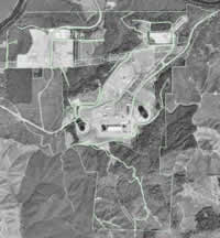
Figure 3.2: Orthophotograph of Satsop Forest
with stand boundaries
(For a larger image, click here.)
Figure 3.3: Map of Satsop Forest cover types.
(For a larger image, click here)
Figure 3.4: Map of Site Classes on Satsop
Forest
(For a larger image, click here)
Figure 3.5: Map of age classes on Satsop
Forest
(For a larger image, click here)
Figure 3.6: map of species distribution on
Satsop Forest
(For a larger image, click here)
Results
There are three components to the results:
- The validation of the models, comparing outputs from the HEP
implemented in LMS with the original results from the original
HEP.
- A set of landscape simulations.
- A set of silvicultural pathways simulated on four individual
stands.
The latter are two are examples of how the HEP implemented in
LMS can be used to assess changes in habitat and timber volumes
caused by different silvicultural pathways from both the landscape-
and stand-level perspectives.
Validation
To assess the performance of the models implemented in LMS, it
was necessary to use data, both tree-based and non-tree-based, from
the original HEP to calculate HSI values for the four species. When
compared with the HSI values calculated during the original HEP
differences range from -0.009 to 0.001. A paired t-test on the differences
between HSI values reported the original HEP and those calculated
with LMS using data from the original HEP was performed using the
statistical analysis software package SPSS 10.0. Mean differences
range from 0.000 - 0.001 with all 95% confidence intervals containing
0.0 (Figure 4.1). Results from the Cooper's hawk HSI model, using
the original HEP data, could not be analyzed using the t-test because
the model predicted the exact HSI values that were reported in the
original HEP analysis. The resulting mean difference of 0.0 with
a standard error of the mean of 0.0 does not allow the paired t-test
to be used. Since all 95% confidence intervals contain 0.0 the models
predict as well as the original HSI models at the 0.05 level.
A second analysis was performed using forest inventory collected
in 1998. A second paired t-test was performed comparing the mean
differences between the HSI values reported in the original HEP
and the HSI values calculated using LMS with this updated data set.
Mean differences ranged from -0.0615 to 0.1176 with all 95% confidence
intervals containing 0.0 (Figure 4.2). Using the updated data made
no significant difference in model outputs at the 0.05 level.
Given these results it can be said that the HSI models, as implemented
in LMS, predicted HSI values as well as the original HSI models
and using updated forest inventory data summarized on a per stand
basis made no significant difference in HSI values for each cover
type.
Landscape Simulations
Landscape simulations yielded a range of effects on both habitat
values and harvested volumes. HU values for Cooper's hawk began
at 343.8 or 305.7 in 1998 and declined during the simulation period.
Southern red-backed vole HU values began at 308.7, 309.0 or 276.9
and increased at varying rates to 481.1 - 682.5. Spotted towhee
HU values began at 122.7 - 127.9 and declined to 16.8 - 67.6. Pileated
woodpecker HU values began at 266.7 - 269.9, then generally increased
to 261.3 - 625.5 (Table 4.1).
Flows of these habitats may be more important than looking at individual
years (Figure 4.3). Generally, Cooper's hawk and spotted towhee
habitat units declined during the entire simulation period, while
southern red-backed vole and pileated woodpecker habitat units increased.
The exception to this is the "timber intensive" simulation
where pileated woodpecker declined.
Harvested volumes varied greatly among the management alternatives
simulated (Table 4.2). Total harvest ranged from 0mbf/yr in the
"no action" alternative to 914.4mbf/yr with the "45-year
rotation" alternative. Sizes of trees harvested varied between
alternatives as well. The greatest proportion of volume was pole
timber under the "moderate enhancement" alternative (42%),
while the greatest proportion of volume of sawlogs was under the
"45-year rotation" alternative (67%), and the greatest
proportion of volume of large sawlogs was under the "intensive
enhancement" alternative (26%).
Flows of harvested volume changed between alternatives as well (Figure
4.4). With the "45-year rotation" alternative, harvested
volume was greatest but the type of harvest changed from a mix of
size classes in the first 45 years to predominantly small sawlogs
in the last 35-years. The "moderate enhancement" alternative
produced very little volume with all the volume concentrated between
2018 and 2038 in pole and small sawlogs. "Intensive enhancement"
yields less total volume than the 45-year rotation, but the distribution
of size classes harvested changed from predominantly pole and small
sawlogs in the first half of the simulation to a majority of the
harvest in large sawlogs in the second half of the simulation. "Mixed
management" yielded fluctuating harvested volumes with the
majority of the volume in the small sawlog size class.
Pathway Simulations
Using the set of silvicultural pathways to assess the effects on
both habitat and harvested volumes on individual stands allows comparisons
among pathways that may be used to promote certain types of habitat.
Sets of 21 pathways applied to two 10-year-old stands, with approximately
435 and 1300tpa, respectively, and sets of 30 pathways simulated
using two 90-year-old stands, one a relatively open single-storied
stand and the other a multiple-storied stand were simulated to assess
yields of habitat qualities and harvested volumes.
Young Stands
The set of 30 silvicultural pathways simulated using data from the
two young stands results in a wide range of HSI values for each
species (Tables 4.3 and 4.4). The greatest average HSI values produced
are for the southern red-backed vole at 0.863 and 0.820 for dense
and open stands, respectively. Silvicultural pathways that produced
the highest habitat values for the vole had light thinnings, from
a single thinning at 10 - 30 years to multiple thinnings during
the 80-year simulation period. Similarly, pileated woodpecker HSI
models respond well to light thinnings in a dense stands. In contrast,
when the open stand was simulated, the woodpecker HSI model responded
best to heavier thinnings at 15 years, but only slightly better
than the light thinnings. In contrast to the responses of the vole
and woodpecker HSI models, the Cooper's hawk HSI model responds
best to heavier thinnings in both dense and open stands and the
spotted towhee model responds best to 40-year rotations and pathways
that simulate "traditional" industrial forest management
approaches. The results from the towhee model are low HSI values
ranging from 0.012 - 0.096.
Both dense and open stands produced the highest total harvest volume
using silvicultural pathways with 40 - 80-year rotations with one
or two intermediate thinnings that mimic "traditional"
forest management practices (Table 4.7). Maximum total volumes produced
were 260 and 216mbf/ac for dense and open stands, respectively.
Average volumes produced by the set of silvicultural pathways were
low at 96 and 80 mbf/ac for the entire simulation period. Silvicultural
pathways focusing on thinnings for habitat development rather than
on harvested volume caused lower average harvested volumes.
Older Stands
The set of 21 silvicultural pathways simulated using data from the
90-year old, single and multiple-storied stands also produce a wide
range of HSI values (Tables 4.5 and 468). As with the young stand
simulations, the vole model produced the greatest average HSI values
of 0.746 and 0.817 for single and multiple storied stands, respectively.
The best model response was to very light thinnings or no action
for both stand structures. The woodpecker model responded very well
to pathways with light thinnings or no action as well. Pathways
with heavier thinnings produced better responses from the hawk model
than the vole or woodpecker models but many of the pathways that
produced the best responses with the hawk model were light thinning
or no action pathways. In contrast to the vole, hawk, and woodpecker
models the towhee model responded best to heavier harvesting in
older stands. As with the young stand simulations the overall response
was low producing HSI values ranging from 0.000 - 0.105.
Highest total harvested volumes were produced with 80-year rotation
pathways leaving two to eight trees per acre from the original stand
(Table 4.7). Total harvest volumes were 248 and 216 mbf/ac, for
single and multiple storied stands, respectively, for the full 80-year
simulation period. Average harvested volumes were low at 94 and
99 mbf/ac. As with the young stands pathway simulations these volumes
are low because the simulated pathways focus on multiple thinnings
for habitat development rather than harvest volume.
Figure 4.1: Mean difference between HSI values reported in
original HEP and values calculated by LMS using original HEP data,
with 95% confidence intervals.
Figure 4.2: Mean difference between HSI values reported in
original HEP and values calculated by LMS using 1998 Satsop Forest
inventory data, with 95% confidence intervals.
|
Table 4.1: Habitat units for all
species modeled for 1998, 2038 and 2078
|
| |
Cooper's hawk
|
Southern red-backed vole
|
Spotted towhee
|
Pileated
woodpecker
|
| Scenario |
1998
|
2038
|
2078
|
1998
|
2038
|
2078
|
1998
|
2038
|
2078
|
1998
|
2038
|
2078
|
| 1. No Action |
343.8
|
309.2
|
277
|
308.7
|
507.9
|
540.8
|
127.9
|
25.6
|
17.5
|
269.9
|
519.6
|
571.3
|
| 2. 45-yr rotation |
343.8
|
99.6
|
98.6
|
308.7
|
453.8
|
481.1
|
127.9
|
70.5
|
67.6
|
269.9
|
209.7
|
216.3
|
| 3. Moderate enhancement |
343.8
|
309.2
|
277
|
308.7
|
508.4
|
540.8
|
127.9
|
25.6
|
17.5
|
269.9
|
534.5
|
571.5
|
| 4. Intensive enhancement |
305.7
|
143.1
|
123.2
|
276.9
|
597.7
|
682.5
|
124.1
|
36.7
|
16.8
|
266.7
|
507.4
|
625.7
|
| 5. Mixed management |
343.8
|
235.7
|
224.8
|
309
|
406.4
|
515.2
|
122.7
|
42.7
|
27.9
|
269.9
|
375.3
|
427.5
|
Figure 4.3: Habitat flows for landscape simulations
Figure 4.3 (continued): Habitat flows for landscape simulations
|
Table 4.2: Annual average harvested
volumes (mbf/yr) and percentage in each size class from landscape
simulations. Pole = <12"dbh, Sawlog = 12-24"dbh, Large Sawlog
= >24"dbh
|
|
Scenario
|
Pole
|
Sawlog
|
Large Sawlog
|
Total
|
|
mbf/yr
|
%
|
mbf/yr
|
%
|
mbf/yr
|
%
|
mbf/yr
|
| 1. No Action |
0.0
|
NA
|
0.0
|
NA
|
0.0
|
NA
|
0.0
|
| 2. 45-yr rotation |
91.8
|
10%
|
611.5
|
67%
|
211.1
|
23%
|
914.4
|
| 3. Moderate enhancement |
19.7
|
42%
|
27.4
|
58%
|
0.0
|
0%
|
47.1
|
| 4. Intensive enhancement |
73.3
|
15%
|
280.5
|
59%
|
124.7
|
26%
|
478.4
|
| 5. Mixed management |
19.7
|
6%
|
273.8
|
81%
|
44
|
13%
|
337.5
|
Figure 4.4: Harvested volumes by size class for five-year projection
periods
4.4 (continued): Harvested volumes by size class for five-year
projection periods
|
Table 4.3: HSI values and top five
pathways for individual pathway simulations using young dense
stand
|
| |
Hawk
|
Vole
|
Woodpecker
|
Towhee
|
| Max |
0.614
|
0.968
|
0.651
|
0.078
|
| Min |
0.2
|
0.58
|
0.112
|
0.012
|
| Average |
0.383
|
0.863
|
0.486
|
0.024
|
| Top five pathways |
Barbour15-150 |
Barbour30-250 |
YSTD-Light |
Hansen0-40 |
| Barbour30-150HL |
YSTD-Light |
BarbourNT |
CC40_PCT |
| Barbour30-75 |
BarbourNT |
Hansen0-120 |
CC60_PCT_CT |
| Barbour15-75 |
Hansen0-120 |
Barbour30-250 |
Hansen0-80 |
| Barbour30-150 |
CareyBDPS |
0_NA |
CC80_PCT_2CT |
|
Table 4.4: HSI values and top five
pathways for individual pathway simulations using young open
stand
|
| |
Hawk
|
Vole
|
Woodpecker
|
Towhee
|
| Max |
0.628
|
0.937
|
0.635
|
0.096
|
| Min |
0.213
|
0.525
|
0.06
|
0.03
|
| Average |
0.437
|
0.82
|
0.408
|
0.048
|
| Top five pathways |
Barbour30-75 |
0_NA |
Barbour15-75 |
Hansen0-40 |
| Barbour30-150HL |
Mit_SOP |
Barbour15-150 |
CC40_PCT |
| CareyBDPF |
McComb_PR |
BarbourNT |
CC60_PCT_CT |
| Barbour30-150 |
CareyBDPS |
YSTD-Light |
Hansen0-80 |
| YSTD-Heavy |
Hansen0-120 |
Barbour30-250 |
CC80_PCT_2CT |
|
Table 4.5: HSI values and top five
pathways for individual pathway simulations using old single
storied stand
|
| |
Hawk
|
Vole
|
Woodpecker
|
Towhee
|
| Max |
0.723
|
0.967
|
0.792
|
0.105
|
| Min |
0.257
|
0.086
|
0
|
0
|
| Average |
0.452
|
0.746
|
0.421
|
0.028
|
| Top five pathways |
DEMO40 |
Hansen150-40 |
Hansen150-120 |
DEMO20 |
| Hansen50-40 |
Hansen150-80 |
Hansen150-80 |
McCombSS |
| McCombMS |
Hansen150-120 |
Hansen150-40 |
Hansen10-40 |
| 0_NA |
0_NA |
0_NA |
Hansen5-40 |
| Hansen150-40 |
Hansen50-120 |
Hansen50-120 |
Hansen15-40 |
|
Table 4.6: HSI values and top five
pathways for individual pathway simulations using old multiple
storied stand
|
| |
Hawk
|
Vole
|
Woodpecker
|
Towhee
|
| Max |
0.644
|
0.976
|
0.914
|
0.08
|
| Min |
0.261
|
0.605
|
0
|
0
|
| Average |
0.419
|
0.817
|
0.492
|
0.027
|
| Top five pathways |
Hansen50-40 |
McCombMS |
0_NA |
McCombSS |
| McCombMS |
DEMO40 |
DEMO40 |
Hansen5-40 |
| Hansen30-40 |
0_NA |
Hansen150-120 |
Hansen10-40 |
| DEMO20 |
DEMO20 |
Hansen150-80 |
CC60_PCT_CT |
| Hansen150-40 |
Hansen150-40 |
McCombMS |
CC40_PCT |
|
Table 4.7: Total harvested volumes
(mbf/ac) and top five pathways for individual pathway simulations
using young-open, young-dense, old-single-story, and old-multiple-story
stands
|
| |
Young-open
|
Young-dense
|
Old-single-story
|
Old-multiple-story
|
| Max |
216
|
260
|
248
|
216
|
| Min |
0
|
0
|
0
|
0
|
| Average |
80
|
96
|
94
|
99
|
| Top Five Pathways |
Hansen0-80 |
Hansen0-80 |
Hansen5-80 |
Hansen5-80 |
| McComb_CC |
McComb_CC |
Hansen10-80 |
Hansen10-80 |
| CC80_PCT_2CT |
CC80_PCT_2CT |
Hansen15-80 |
Hansen15-80 |
| CC40_PCT |
CC40_PCT |
Hansen20-80 |
Hansen20-80 |
| Hansen0-40 |
Hansen0-40 |
McCombSS |
McCombSS |
Discussion and Management Applications
Discussion of this approach to habitat assessment and applications
to management is presented in four components:
- Habitat model responses
- Management applications
- Advantages of integrating the HEP and LMS
- Limitations of integrating the HEP and LMS
Habitat Model Responses
Each species' HSI model responds differently in response to the
simulated management scenarios. From a landscape-level habitat perspective,
Cooper's hawk habitat quantity declined with all simulated management
alternatives, with the more intensive harvesting in the 45-year
rotation and intensive enhancement alternatives causing the largest
declines. The declines are caused by a mortality of shorter-lived
hardwood species, such as red alder, during the simulation with
increased declines with the conversion of hardwood stands to conifer
stands in the 45-year rotation and intensive enhancement alternatives.
Hardwood components of stands are important for the Cooper's hawk
HSI models.
Similarly, spotted towhee habitat quantity declined during the simulation
period because canopy closure increased as the stands grew. The
45-year rotation alternative provided the smallest decline because
harvesting stands at 45 years provided the most early-successional,
open stands used by the spotted towhee for habitat.
Southern red-backed vole habitat quantity increased for all harvest
intensity levels, with the intensive enhancement alternative providing
the most habitat. All alternatives provide trees of sufficient size
and enough canopy closure for the southern red-backed vole HSI model
to respond positively.
Pileated woodpecker habitat quantity generally increased as well,
with the exception of the 45-year rotation alternative. Increases
were caused by the development of stands with larges tree cover
type classifications that provide more, larger snags, stumps and
logs - all of which are important to this HSI model.
Changing to a stand-level perspective changes in habitat quality
caused by different silvicultural pathways can be assessed. Cooper's
hawk HSI values ranged from 0.200 to 0.723 for all pathways simulated,
with an average of 0.423. This range was caused by the changes in
total canopy closure and conifer canopy closure. Since all stands
simulated had >80% of total basal area in conifers, these canopy
closures tended to counteract each other in the calculations, resulting
in lower HSI values.
Southern red-backed voles showed the least sensitivity to different
stand pathways, with a range of HSI values from 0.086 to 0.967 and
an average of 0.811 for all simulations. Here, too the low sensitivity
to harvesting was caused by these pathways providing sufficient
canopy closure and large trees to provide high habitat quality values.
Pileated woodpecker showed great sensitivity to simulated pathways.
Average HSI values ranged from 0.000 to 0.914, with an average 0.452.
Since the model required large trees and snags, the time that the
stand is allowed to grow before harvest and the type of harvest
both affect the resulting HSI values. Since not all of the pathways
allowed stands to attain sufficient large trees, the HSI models
for pileated woodpeckers were generally quite sensitive.
The spotted towhee model showed a similar sensitivity, with HSI
values ranging from 0.105 to 0.000 and an average of 0.032. This
model required low canopy closure for increased quality of shrubs
and ground cover; thus, increased harvest intensity and heavier
thinning provided better results from the model. When stands were
allowed to remain in an open condition longer, the average HSI values
increased.
Management Applications
Given the responses of the HSI models to the various silvicultural
pathways questions should be asked regarding "broad-brush",
single-species, and ecosystem management approaches. Results from
the landscape simulations give insights into the appropriateness
of the "broad-brush" approach of applying a 45-year rotation
to all stands on the landscape. The simulation demonstrated declines
in habitat quantity for all species except the southern red-backed
vole. The loss of habitat comes with the benefit of increased harvested
volume, and hence increased income, over the simulation period.
An alternative to this approach is the Intensive Enhancement landscape
simulation where different silvicultural pathways were applied to
different stands on the landscape. Habitat quantity is increased
for both the vole and pileated woodpecker under this management
regime.
Assessing trade-offs among management objectives is an important
aspect of management planning (Table 5.1). For example, annual average
harvest is at a maximum with a 45-year rotation but it comes at
a cost to wildlife habitat. This management approach reduces Cooper's
hawk and pileated woodpecker habitat the greatest, while reducing
spotted towhee habitat the least. On the other hand, a moderate
approach with minimal thinning can be done to provide good habitat
levels for all species other than the spotted towhee. This comes
at a cost of approximately 867.3 mbf (95% reduction) of harvested
volume per year. Another approach is to implement a system of multiple
thinnings with the intensive enhancement scenario. This provides
very good habitat for both southern red-backed voles and pileated
woodpeckers, but reduces habitat for Cooper's hawks and spotted
towhees. Harvest with this scenario is reduced by 436 mbf/yr (48%).
This may be an acceptable loss of harvested volume to the decision
maker.
Costs associated with providing wildlife habitat can be further
increased by higher logging costs. Leaving more trees in a harvest
unit makes harvesting more difficult, with an associated increase
in logging costs (Kellogg, Pilkerton et al. 1991; Kellogg, Bettinger
et al. 1996; Chambers, McComb et al. 1999).
Some or all of these extra costs may be recovered through other
means. Increased wildlife may bring added revenue through activities
such as wildlife viewing and hunting (Freese and Trauger 2000; Loomis
2000). If wildlife revenues are quantified and related to timber
volumes, areas of stand structures, habitat levels, or other attribute
that can be calculated using LMS this revenue could then be included
into financial analyses within LMS.
Managing for maximum habitat for a single species may not be appropriate
if there are multiple species of concern in an area. As an example,
managing at the landscape level applying the silvicultural pathways
that provided the maximum amount of pileated woodpecker habitat
cam at the expense of spotted towhee habitat. At the stand level
silvicultural pathways that provide high levels of vole or woodpecker
habitat generally provide for lower levels of Cooper's hawk habitat
and little or no spotted towhee habitat. If the intent of management
is to provide habitat for multiple species on the landscape, through
ecosystem management, it will be necessary to apply several different
silvicultural pathways on a landscape to provide a variety of stand
structures and associated habitat values across the landscape.
Assessing trade-offs in habitat and harvest volume was done by in
a hypothesis-testing framework. Compiling all pathways that were
among the five best for each species resulted in twenty pathways
for young stands (Table 5.2). For stands that are initially 10-years
old and with an initial density of approximately 435 tpa, four of
the 20 pathways provided the most habitat for two species - southern
red-backed vole and pileated woodpecker. Thirteen of the remaining
pathways provide the most habitat for a single species - five for
Cooper's hawk and spotted towhee independently, two for pileated
woodpecker, and one for southern red-backed vole. The remaining
three pathways provide the most habitat only with initially dense
stands. For the initially dense 10-year old stand with approximately
1300 tpa, all pathways provided the most habitat for a single species.
Five provided the most habitat for pileated woodpecker, southern
red-backed vole, Cooper's hawk and spotted towhee, independently.
Averaging the habitat for both stands yielded four stands that provide
the most habitat for 1.5 species - Cooper's hawk and southern red-backed
vole either together or independently. Thirteen pathways provide
habitat independently, either Cooper's hawk, southern red-backed
vole, pileated woodpecker, or spotted towhee. Three pathways that
provided the most habitat for an average of 0.5 species, either
Cooper's hawk or southern red-backed vole in half of the pathways.
Compiling pathways for older stands yielded sixteen pathways that
benefited on, or more, species in simulations of single and multiple
story stands (Table 5.3). With an initially single storied stand,
two pathways provided the most habitat for three species, (Cooper's
hawk, southern red-backed vole, and pileated woodpecker), three
pathways that provided the most habitat for two species, (southern
red-backed vole and pileated woodpecker), and eight pathways that
provided the most habitat for a single species, (either Cooper's
hawk or spotted towhee). Three pathways provided the most habitat
only with an initially multiple storied stand. With an initially
multiple storied stand, one pathway provided the most habitat for
three species, (Cooper's hawk, southern red-backed vole, and pileated
woodpecker), six pathways provided the most habitat for two species,
(either southern red-backed vole and pileated woodpecker or southern
red-backed vole and pileated woodpecker), and seven pathways that
provided the most habitat for only a single species, (either spotted
towhee or Cooper's hawk). Two pathways provided the most habitat
only with an initially single storied stand. When averaged, two
pathways provide the most habitat for 2.5 species, (Cooper' hawk
and southern red-backed vole and/or pileated woodpecker), three
pathways provided the most habitat for two species, (southern red-backed
vole and pileated woodpecker and/or Cooper's hawk), two pathways
provided the most habitat for 1.5 species, five pathways provided
the most habitat for a single species and four provided the most
habitat for 0.5 species, on average.
Harvested volume from each pathway can be assessed as well. With
the young stand simulations the average maximum harvested volume
was 238 mbf/ac. Pathway simulations for older stands resulted in
an average total harvested volume of 221.5 mbf/ac. Pathways that
provided the most benefit for the wildlife species can be examined
from the perspective of reduction of harvested volume (Tables 5.4
and 5.5).
Pathways that benefited the most species tended to have lower harvested
volumes. Pathways with higher total harvested volumes tended to
provide the best average habitat for a single species, the spotted
towhee. One exception is the CareyDBPS pathway for young stands.
This pathway provided very good southern red-backed vole habitat
(HSI values of 0.966 and 0.929 for initially open and dense stands,
respectively) as well as good pileated woodpecker habitat (HSI value
of 0.637 and 0.492 for initially open and dense stands, respectively)
and fair Cooper's hawk habitat (HSI values of 0.342 and 0.506 for
initially open and dense stands, respectively).
All these proposed pathways had been intended to produce habitat
as well as allowed some harvesting. Testing them with LMS and the
habitat models allowed the pathways to be simulated on local forest
conditions before they are applied. Since the pathways were proposed
for other regions of the Pacific Northwest and for other stands
conditions the results may be different than reported for the area
that they were developed for. Variations in initial conditions have
an effect on the habitat outputs from the pathways, as can be seen
in the differences between the HSI values for each species when
comparing individual stand pathways on stands with different initial
conditions on Satsop Forest. The number of species benefited is
also dependent on initial conditions. The same pathway may benefit
multiple species with one initial condition while none with another
initial condition. These potential effects can be assessed using
these models in a hypothesis-testing framework to avoid potential
unintended consequences when pathways are implemented in the forest.
After the assessment of habitat and volume trade-offs was completed
the top performing pathways for each species and harvested volume
are used to create landscape-level management alternatives. Selecting
the proportion of the landscape that a particular silvicultural
pathway is applied to is accomplished by grouping stands on the
landscape into ecologically similar groups, simulating all the pathways
using an "average" stand from the group, then using the
Toggle Program to apportion the amounts of each group that receive
particular pathways (Johnson 2001).
Analyzing trade-offs among multiple, often conflicting, objectives
it one of the primary strengths of the Toggle Program. As the user
adjusts the percentage of each group that pathways are applied to,
resultant values of all outputs included in the Toggle Program are
calculated. Outputs include wildlife habitat, sequestered carbon,
standing and harvested volumes by tree size classes, landscape-level
structural diversity, reserve areas, susceptibility to windthrow,
and even potential employment.
Working with the Toggle Program the user develops several management
alternatives. Outputs from each set of silvicultural pathways are
reported in matrix format for side-by-side comparisons of the various
outputs of interest. The resulting matrix can then be given to the
person, or people, in charge of making the final decision regarding
a management plan for a landscape.
Advantages Of Integrating HEP and LMS
Implementing the HEP calculations in LMS provided several advantages.
First, since an empirical growth model is used, all assumptions
are held constant for all forest growth simulations, allowing alternatives
to be compared without bias.
Using a forest inventory allows the variability within each cover
type to be included in the analysis. Based on the cover type classification
rules there can be a wide range of tree sizes and canopy closures
as well as understory, snag and downed wood components. Selecting
only an average tree size or other value, instead of using a forest
inventory, may neglect variability result in lower habitat quality.
Examples of this are the improved results using the 1998 Satsop
Forests inventory instead of the original HSI calculations based
on cover type averages from the original HEP data collection.
The most significant advantage of automating these calculations
in LMS is the ability to develop and analyze many alternatives quickly.
Both landscape level and stand level simulations can be made to
assess and communicate the effects of proposed management regimes.
The rapid analysis is especially important when some parties involved
in planning have backgrounds other than forestry, and so do not
understand standard forestry metrics such as volume, tree sizes
and stands structures. When working at the stand level, several
alternative silvicultural pathways can be compared to assess their
potential benefits. Using hypothesis-testing framework before they
are applied in a whole forest landscape.
Other approaches to habitat assessment over spatial and temporal
scales could be used. For example, using FVS directly, without the
LMS interface, to perform forest growth projections then feeding
the resulting data into the HSI models would result in equivalent
results. Using FVS within LMS adds other dimensions to an analysis.
FVS can provide a set of raw outputs tables that will need further
summarization to perform other analyses. In this analysis only a
small segment of the functionality and power of LMS are used. HSI,
HU, and volume calculations all use only the inventory and stand
attribute files to create output tables.
Many other analyses are available to the user of LMS. Over thirty
analysis tables are included with LMS that are created by programs
within LMS, which summarize the current and projected future inventories
in different ways. Tables created in this process have been developed
to answer questions relating not only to levels of habitat and volumes
but also other forestry measures such as inventory tables and stand
summary tables as well as other measures such as carbon sequestration
and stand structures.
Other assessments include landscape and stand level visualizations
using the Stand Visualization System and EnVision programs, developed
by Robert McGaughey, Research Forester, USDA Forest Service, Pacific
Northwest Research Station, University of Washington, Seattle, WA,
that are included with LMS. Using these assessments of aesthetic
changes to the forest can be performed. Visualizations also allow
the analyst to communicate changes in to forest caused by forest
management activities.
A second approach developing a landscape level management plan uses
the ORGANON growth model in conjunction with a GIS system and the
harvest-scheduling program SNAP-II (McComb, Spies et al. 1993).
This approach differs from the LMS and Toggle Program approach in
one main way: SNAP-II is decision-making program while LMS is a
decision-support program. Through optimization routines with constraints
on various outputs SNAP-II determines an optimal schedule of what
to harvest when and when. Implicit in the ORGANON / SNAP-II approach
is an assumption that the analyst knows the appropriate weighting
levels for the desired outputs creating a top-down approach to decision
making. When using the LMS / Toggle Program approach no assumptions
are made about the importance various objectives. It is up to the
user to select the appropriate mix of pathways. The LMS / Toggle
are used as decision-support tools in the management plan development
process.
Limitations Of Integrating HEP and LMS
This approach also has several limitations. Since understory, snag
and downed wood data are needed for calculating HSI values for all
models except Cooper's hawk, the applicability of these models is
limited to the Satsop Forest ownership without collection of appropriate
understory, snag, and downed wood data. Applying these models elsewhere
would require collection of the appropriate data and calculations
of average values based on cover types classified by the cover type
classification algorithm.
Understory relationships in Pacific Northwest forests have been
studied in great depth. Studies have focused on developing relationships
between overstory and understory structure and composition, as well
as responses of the understory to disturbances, including harvesting,
in old-growth, mature, and young forests (Halpern and Spies 1995;
Bailey, Maysohn et al. 1998; Van Pelt and Franklin 2000). Relationships
have been developed into models for other regions of the Pacific
Northwest (McPherson 1992; Klinka, Chen et al. 1996; Mitchell and
Popovich 1997), but none were found for Southwest Washington, where
Satsop Forest is located. Forest inventory that is limited to tree
measures will have little success in estimating wildlife habitat
using the framework of this paper, since both the spotted towhee
and southern red-backed vole require understory metrics as well
as tree metrics. Development of understory models for other regions
shows that it can be done, and building models for Western Washington
would increase the applicability of the models to other areas of
the region.
Snags and downed wood are important habitat attributes for pileated
woodpecker and southern red-backed vole models. The current version
of LMS, version 2.0.42h, does not model snags and downed wood. Earlier
versions had included a snag and downed wood model. A snag and downed
wood model is scheduled for release with the next version of LMS.
Application of this model will allow the models to estimate habitat
with variability of snags and downed wood within each cover type
included. It is hoped that including snag and downed wood in the
models will increase their sensitivity in the same way as using
the 1998 Satsop Forest inventory rather than the original cover
type averages.
Creation of snags through various methods has been proposed to provide
habitat for cavity-nesters where insufficient snags are present
(Lewis 1998). Use of these snags has been noticed where they have
been created in commercial forests (Chambers, Carrigan et al. 1997).
Creation of snags and downed wood, however, cannot be simulated
with the current version of LMS. Inclusion of this snag creation
along with the snag and downed wood model with the next version
of LMS will also allow estimation of the benefit provided by creation
of these structures in managed forest landscapes.
Spatial arrangement and size of habitat patches is important for
some species. Pileated woodpeckers need a home range of at up to
600ac (Schroeder 1983). In the case of Satsop Forest, with an average
polygon (habitat patch) size of 5.2ac, the ability to arrange harvest
activities is such a way that minimum home range requirements are
met is through iterative applications of silvicultural pathways
to various stands. After an initial management plan simulation,
there may be 600ac of pileated woodpecker habitat but it may be
arranged in a series of small patches that are not of use for the
woodpeckers. This is less of a concern for a species with a small
home range such as the southern red-backed vole with a home range
size of up to approximately 3.5ac (Allen 1983).
Adaptive Management
These models should be used in an adaptive management context as
well. Growth model outputs are only a representation of what may
exist in the future. It is necessary to revisit the results after
several years to ensure that the silvicultural pathways are providing
the desired results. If the silvicultural pathways are not producing
the desired habitat results the pathways can be modified to produce
the needed habitat structures.
The HSI models do not provide actual species populations, only measures
of potential habitat quality and quantity. Thus it will be necessary
to perform field surveys in the future to determine if animals are
actually using the habitats that are expected to exist on the landscape.
If species are using habitats different from the model's predictions,
the models may be modified using the monitoring data to predict
habitat suitability indices better. This may also allow relationships
between HSI values and actual populations numbers to be developed.
|
Table 5.1: Comparison of annual harvested
volumes (mbf/yr) to percent changes in wildlife habitat over
an 80-year simulation (bold = maximum, italics = minimum)
|
| |
Annual harvest (mbf/yr)
|
Cooper's hawk
|
Southern red-backed vole
|
Pileated woodpecker
|
Spotted towhee
|
| |
2038
|
2078
|
2038
|
2078
|
2038
|
2078
|
2038
|
2078
|
| 1. No Action |
0
|
-10%
|
-19%
|
65%
|
75%
|
93%
|
112%
|
-80%
|
-86%
|
| 2. 45-yr rotation |
914.4
|
-71%
|
-71%
|
47%
|
56%
|
-22%
|
-20%
|
-45%
|
-47%
|
| 3. Moderate enhancement |
47.1
|
-10%
|
-19%
|
65%
|
75%
|
98%
|
112%
|
-80%
|
-86%
|
| 4. Intensive enhancement |
478.4
|
-53%
|
-60%
|
116%
|
146%
|
90%
|
135%
|
-70%
|
-86%
|
| 5. Mixed management |
337.5
|
-31%
|
-35%
|
32%
|
67%
|
39%
|
58%
|
-65%
|
-77%
|
|
Table 5.2: Twenty pathways with highest
average HSI values over an 80 year simulation for stands initially
10-years old, open (~435 tpa) and dense (~1300 tpa), with
species benefited (CH = Cooper's hawk, SRV = southern red-backed
vole, PW = pileated woodpecker, ST = spotted towhee)
|
|
Pathway
|
Open
|
Dense
|
Average
|
Open
|
Dense
|
| Barbour30-250 |
2
|
1
|
1.5
|
SRV, PW
|
PW
|
| BarbourNT |
2
|
1
|
1.5
|
SRV, PW
|
PW
|
| Hansen0-120 |
2
|
1
|
1.5
|
SRV, PW
|
SRV
|
| YSTD-Light |
2
|
1
|
1.5
|
SRV, PW
|
PW
|
| 0_NA |
1
|
1
|
1
|
PW
|
SRV
|
| Barbour15-150 |
1
|
1
|
1
|
CH
|
PW
|
| Barbour15-75 |
1
|
1
|
1
|
CH
|
PW
|
| Barbour30-150 |
1
|
1
|
1
|
CH
|
CH
|
| Barbour30-150HL |
1
|
1
|
1
|
CH
|
CH
|
| Barbour30-75 |
1
|
1
|
1
|
CH
|
CH
|
| CareyBDPS |
1
|
1
|
1
|
SRV
|
SRV
|
| CC40_PCT |
1
|
1
|
1
|
ST
|
ST
|
| CC60_PCT_CT |
1
|
1
|
1
|
ST
|
ST
|
| CC80_PCT_2CT |
1
|
1
|
1
|
ST
|
ST
|
| Hansen0-40 |
1
|
1
|
1
|
ST
|
ST
|
| Hansen0-80 |
1
|
1
|
1
|
ST
|
ST
|
| Mit_SOP |
1
|
1
|
1
|
PW
|
SRV
|
| McComb_PR |
0
|
1
|
0.5
|
|
SRV
|
| CareyBDPF |
0
|
1
|
0.5
|
|
CH
|
| YSTD-Heavy |
0
|
1
|
0.5
|
|
CH
|
|
Table 5.3: Sixteen pathways with
highest average HSI values over an 80 year simulation for
stands initially 90-years old, single and multiple layered
canopy, with species benefited (CH = Cooper's hawk, SRV =
southern red-backed vole, PW = pileated woodpecker, ST = spotted
towhee)
|
|
Pathway
|
Single
|
Multiple
|
Average
|
Single
|
Multiple
|
| 0_NA |
3
|
2
|
2.5
|
CH, SRV, PW |
SRV, PW |
| Hansen150-40 |
3
|
2
|
2.5
|
CH, SRV, PW |
CH, SRV |
| Hansen150-120 |
2
|
2
|
2
|
SRV, PW |
SRV, PW |
| Hansen150-80 |
2
|
2
|
2
|
SRV, PW |
SRV, PW |
| McCombMS |
1
|
3
|
2
|
CH |
CH, SRV, PW |
| DEMO20 |
1
|
2
|
1.5
|
ST |
CH, SRV |
| DEMO40 |
1
|
2
|
1.5
|
CH |
SRV, PW |
| Hansen50-120 |
2
|
0
|
1
|
SRV, PW |
|
| Hansen10-40 |
1
|
1
|
1
|
ST |
ST |
| Hansen5-40 |
1
|
1
|
1
|
ST |
ST |
| Hansen50-40 |
1
|
1
|
1
|
CH |
CH |
| McCombSS |
1
|
1
|
1
|
ST |
ST |
| Hansen15-40 |
1
|
0
|
0.5
|
ST |
|
| CC40_PCT |
0
|
1
|
0.5
|
|
ST |
| CC60_PCT_CT |
0
|
1
|
0.5
|
|
CH |
| Hansen30-40 |
0
|
1
|
0.5
|
|
CH |
|
Table 5.4: Total harvested volume
(mbf/ac) from an initially 10-year old stand during an 80-year
simulation for 16 top habitat-producing pathways and species
benefited (CH = Cooper's hawk, SRV = southern red-backed vole,
PW = pileated woodpecker, ST = spotted towhee.)
|
|
Pathway
|
Open
|
Dense
|
Average
|
Open
|
Dense
|
| Barbour30-250 |
34
|
41
|
37.5
|
SRV, PW |
PW |
| BarbourNT |
4
|
5
|
4.5
|
SRV, PW |
PW |
| Hansen0-120 |
3
|
4
|
3.5
|
SRV, PW |
SRV |
| YSTD-Light |
37
|
44
|
40.5
|
SRV, PW |
PW |
| 0_NA |
0
|
0
|
0
|
PW |
SRV |
| Barbour15-150 |
26
|
32
|
29
|
CH |
PW |
| Barbour15-75 |
22
|
27
|
24.5
|
CH |
PW |
| Barbour30-150 |
46
|
55
|
50.5
|
CH |
CH |
| Barbour30-150HL |
56
|
67
|
61.5
|
CH |
CH |
| Barbour30-75 |
56
|
67
|
61.5
|
CH |
CH |
| CareyBDPS |
126
|
151
|
138.5
|
SRV |
SRV |
| CC40_PCT |
155
|
185
|
170
|
ST |
ST |
| CC60_PCT_CT |
139
|
166
|
152.5
|
ST |
ST |
| CC80_PCT_2CT |
170
|
204
|
187
|
ST |
ST |
| Hansen0-40 |
147
|
177
|
162
|
ST |
ST |
| Hansen0-80 |
216
|
260
|
238
|
ST |
ST |
| Mit_SOP |
34
|
41
|
37.5
|
PW |
SRV |
| McComb_PR |
57
|
69
|
63
|
|
SRV |
| CareyBDPF |
105
|
126
|
115.5
|
|
CH |
| YSTD-Heavy |
66
|
80
|
73
|
|
CH |
|
Table 5.5: Total harvested volume
(mbf/ac) from an initially 90-year old stand during an 80-year
simulation for the 16 top habitat-producing pathways and the
species benefited (CH = Cooper's hawk, SRV = southern red-backed
vole, PW = pileated woodpecker, ST = spotted towhee.)
|
|
Pathway
|
single
|
multi
|
Average
|
single
|
multi
|
| 0_NA |
0
|
0
|
0
|
CH, SRV, PW |
SRV, PW |
| Hansen150-40 |
0
|
2
|
1
|
CH, SRV, PW |
CH, SRV |
| Hansen150-120 |
0
|
1
|
0.5
|
SRV, PW |
SRV, PW |
| Hansen150-80 |
0
|
8
|
4
|
SRV, PW |
SRV, PW |
| McCombMS |
48
|
10
|
29
|
CH |
CH, SRV, PW |
| DEMO20 |
42
|
0
|
21
|
ST |
CH, SRV |
| DEMO40 |
24
|
0
|
12
|
CH |
SRV, PW |
| Hansen50-120 |
61
|
11
|
36
|
SRV, PW |
|
| Hansen10-40 |
148
|
113
|
130.5
|
ST |
ST |
| Hansen5-40 |
166
|
127
|
146.5
|
ST |
ST |
| Hansen50-40 |
36
|
33
|
34.5
|
CH |
CH |
| McCombSS |
181
|
143
|
162
|
ST |
ST |
| Hansen15-40 |
127
|
99
|
113
|
ST |
|
| CC40_PCT |
152
|
118
|
135
|
|
ST |
| CC60_PCT_CT |
128
|
100
|
114
|
|
CH |
| Hansen30-40 |
78
|
64
|
71
|
|
CH |
Conclusions
Managing forests for wildlife habitats and timber harvest simultaneously
requires assessing habitats and harvest at a landscape level. "Landscapes"
range from a few stands of several acres to ownerships of hundreds
or thousands of acres to watersheds or regions. The common element
in developing management plans is looking at multiple stands in
a landscape as the analysis unit rather than an individual stand.
Performing analyses at this level is necessary for habitat assessment
because animals may have home ranges much larger than a single stand.
Furthermore, in an area there may be more than one species of concern
requiring different management strategies. By moving to analyses
at a landscape level trade-offs between habitat areas may be noticed
and management plans tailored to the needs of multiple species rather
than a single species. LMS is well suited for this type of analysis
because it integrates data at a landscape level and performs landscape
level simulations.
Stand level simulations can also be performed in LMS to assess how
well alternative silvicultural pathways perform in local forests.
Pathways that were proposed for a forest in a different region may
not provide the same habitat values when moved to a different region
with a similar forest type. Reasons for the non-transferability
include differences in site quality, species mixtures, stand ages,
and stand structures. Using LMS these pathways can be tested to
assess if they are appropriate for a specific stand type before
they are applied in the forest. Performing this analysis prior to
application may help to avoid potential unintended consequences.
Analyses in this study have used only a portion of the functionality
of LMS. Many output tables are available that calculate typical
forestry metrics such as basal area and volumes, economic values,
as well as ecological metrics such as canopy layers and stand structural
stages. This study has expanded the set of tables to include wildlife
habitats. The range of tables allows analysts to perform trade-off
analyses from a variety of perspectives. In addition to the tabular
output stand and landscape level visualizations can be produced
using the Stand Visualization System and EnVision programs. Tabular
data are primarily useful for forestry and wildlife professionals
but are difficult for people without train to understand. Visualizations
are one way to help communicate effects of silvicultural treatments
to people involved in the planning process. Through integrative,
analytical, and communicative functions, LMS can be used as an effective
decision support and forest-planning tool.
Bibliography
Allen, A. W. (1983). Habitat suitability index models: Southern
red-backed vole (western U.S.), USDI Fish and Wildlife Service:
14.
Bailey, J. D., C. Maysohn, et al. (1998). "Understory vegetation
in old and young Douglas-fir forests of western Oregon." Forest
Ecology and Management 112: 289-302.
Baker, P. J. and J. S. Wilson (2000). "A quantitative technique
for the identification of canopy stratification in tropical and
temperate forests." Forest Ecology and Management 127: 77-86.
Barbour, R. J., S. Johnston, et al. (1997). "Simulating stand
characteristics and wood product yields from Douglas-fir plantations
managed for ecosystem objectives." Forest Ecology and Management
91(1997): 205-219.
Bevers, M. and J. Hof (1999). "Spatially optimizing wildlife
habitat edge effects in forest management linear and mixed-integer
programs." Forest Science 45(2): 249-258.
Carey, A. B., C. Elliot, et al. (1996). Washington Forest Landscape
Management Project - a pragmatic, ecological approach to small landscape
management, Report No. 2. Olympia, WA, Washington State Department
of Natural Resources: 99 p.
CCEM (1993). Communique: Young managed stands. Corvallis, OR, Cascade
Center for Ecosystem Management, Oregon State University: 16 p.
Chambers, C. L., T. Carrigan, et al. (1997). "Use of artificially
created Douglas-fir snags by cavity nesting birds." Western
Journal of Applied Forestry 12(3): 93-97.
Chambers, C. L., W. C. McComb, et al. (1999). "CFIRP: What
we have learned in the first ten years." The Forestry Chronicle
75(3): 431-434.
Crookston, N. L. and A. R. Stage (1999). Percent canopy closure
and stand structure statistics from the Forest Vegetation Simulator.
Gen Tech. Rep. RMRS-GTR-24. Ogden, UT, USDA Forest Service, Rocky
Mountain Research Station: 11 p.
DeBell, D. S. and R. O. Curtis (1993). "Silviculture and new
forestry in the Pacific Northwest." Journal of Forestry 91(12):
25-30.
Donnelley, D. M. (1997). Pacific Northwest variant of the Forest
Vegetation Simulator. Fort Collins, CO, USDA Forest Service Forest
Management Service Center: 52.
Freese, C. H. and D. L. Trauger (2000). "Wildlife markets
and biodiversity conservation in North America." Wildlife Society
Bulletin 28(1): 42-51.
Halpern, C. B. and T. A. Spies (1995). "Plant species diversity
in natural and managed forest of the Pacific Northwest." Ecological
Applications 5(4): 913-934.
Hann, D. W., C. L. Olsen, et al. (1994). ORGANON user's manual:
Edition 4.3, Southwest Oregon version, and edition 1.3, Western
Willamette Valley version. Corvallis, OR, Oregon State University,
Department of Forest Resources: 113 pp.
Hansen, A. J., S. L. Garman, et al. (1995). "Alternative silvicultural
regimes in the Pacific Northwest: Simulations of ecological and
economic results." Ecological Applications 5(3): 535-554.
Johnson, M. C. (2001). A practical approach to developing a forest
management plan using the Landscape Management System & its
companion programs ("Scope & Group" & "Toggle")
and the rational iterative decision making process. College of Forest
Resources. Seattle, WA, University of Washington.
Kellogg, L. D., P. Bettinger, et al. (1996). "A comparison
of logging planning, felling, and skyline yarding costs between
clearcutting and five group-selection harvesting methods."
Western Journal of Applied Forestry 11(3): 90-96.
Kellogg, L. D., S. J. Pilkerton, et al. (1991). Logging requirements
to meet new forestry prescriptions. COFE Annual Meeting, Nanimo,
British Columbia, Canada, Faculty of Forestry, University of British
Columbia, Vancouver, Canada.
King, J. E. (1966). Site-index curves for Douglas-fir in the Pacific
Northwest. Centralia, WA, Weyerhaeuser Forestry Research Center:
49.
Klinka, K., H. Y. Chen, et al. (1996). "Forest canopies and
their influence on understory vegetation in early-seral stands on
western Vancouver Island." Northwest Science 70(3): 193-200.
Kliskey, A. D., E. C. Lofroth, et al. (1999). "Simulating
and evaluating alternative resource-use strategies using GIS-based
habitat suitability indices." Landscape and Urban Planning
45(1999): 163-175.
Lewis, J. C. (1998). "Creating snags and wildlife trees in
commercial forest landscape." Western Journal of Applied Forestry
13(3): 97-101.
Loomis, J. B. (2000). "Can environmental economic valuation
techniques aid ecological economics and wildlife conservation?"
Wildlife Society Bulletin 28(1): 52-60.
McCarter, J. B., J. S. Wilson, et al. (1998). "Landscape management
through integration of existing tools and emerging technologies."
Journal of Forestry 96(6): p. 17-23.
McComb, W. C., T. A. Spies, et al. (1993). "Douglas-fir Forests:
Managing for Timber and Mature Forest Habitat." Journal of
Forestry 91(12): 31-42.
McPherson, G. R. (1992). "Comparison of linear and non-linear
understory models for ponderosa pine: a conceptual framework."
Forest Ecology and Management 55: 31-34.
Michaelis, L. O. (2000). Assuring a future for private timber management.
Summit 2000: Washington Private Forests Forum, Olympia, WA, Institute
of Forest Resources.
Mitchell, J. E. and S. J. Popovich (1997). "Effectiveness
of basal area for estimating canopy cover of ponderosa pine."
Forest Ecology and Management 95(45-51).
Moore, C. T., M. J. Conroy, et al. (2000). "Forest management
decisions for wildlife objectives: System resolution and optimality."
Computers and Electronics in Agriculture 27(2000): 25-39.
Reineke, L. H. (1933). "Perfecting a stand-density index for
even-aged forests." 46: 627-638.
Rempel, R. S., P. C. Elkie, et al. (1997). "Timber management
and natural-disturbance effects on moose habitat: landscape evaluation."
Journal of Wildlife Management 61(2): 517-524.
Schroeder, R. L. (1983). Habitat suitability index models: Pileated
woodpecker. Washington, DC, USDI Fish and Wildlife Service: 26 p.
Urban, D. L. (1992). ZELIG 2.0: notes on upgrades from version
1.0. Fort Collins, CO, USA, Colorado State University.
USDI (1978). Habitat suitability index model: Spotted towhee, Fish
and Wildlife Service: 4 p.
USDI (1980a). Habitat evaluation procedures 102 ESM. Washington,
DC, USDI Fish and Wildlife Service.
USDI (1980b). Habitat as a basis for environmental assessment,
101 ESM. Washington, DC, UDSI Fish and Wildlife Service.
USDI (1980c). Habitat suitability index model: Cooper's hawk. Washington,
DC, Fish and Wildlife Service: 8 p.
Van Dyck, M. G. (2001). Keyword reference guide for the Forest
Vegetation Simulator. Fort Collins, CO, Forest Management Service
Center, USDA Forest Service: 96 p.
Van Pelt, R. and J. F. Franklin (2000). "Influences of canopy
structure on the understory environment in tall, old-growth, conifer
forests." Canadian Journal of Forestry Research 30: 1231-1245.
WDFW (1991). Black-tailed deer (Odocoileus hemionos columbianus)
winter habitat evaluation model for Western Washington (post workshop
draft). Olympia, WA, Washington State Department of Fish and Wildlife.
WPPSS (1994a). Satsop Power Plant Habitat Evaluation Procedure
(HEP) Analysis. Elma, WA, Washington Public Power Supply System:
22.
WPPSS (1994d). Appendix N: Model habitat unit outputs: Satsop Power
Plant Habitat Evaluation Procedure (HEP) Analysis. Elma, WA, Washington
Public Power Supply System: 22.
WPPSS (1994e). Satsop Power Plant Site wildlife mitigation plan,
revision 1. Elma, WA, Washington Public Power Supply System: 8.
WPPSS (1994f). Satsop Power Plant wildlife mitigation plan standard
operating procedures. Elma, WA, Washington Public Power Supply System:
27 p.
WSEFSEC (1990). Resolution No. 254. Olympia, WA, Washington State
Energy Facility Site Evaluation Council.
|