|
 |
 |
 |


Chapter 2. Measurements of Logs
Chapter 2. Table of Content
|
|||||||||||||||||||||||||||||||||||||||||||||||||||||||||||||||||||||||||||||||||||||||||||||||||||||||||||||||||||||||||||||||||||||||||||||||||||||||||||||||||||||||||||||||||||||||||||||||||||||||||||||||||||||||||||||||||||||||||||||||||||||||||||||||||||||||||||||||||||||||||||||||||||||||||||||||||||||||||||||||||||||||||||||||||||||||||||||||||||||||||||||||||||||||||||||||||||||||||||||||||||||||||||||||||||||||||||||||||||||||||||||||||||||||||||||||||||||||||||||||||||||||||||||||||||||||||||||||||||||||||||||||||||||||||||||||||||||||||||||||||||||||||||||||||||||||||||||||||||||||||||||||||||||||||||||||||||||||||||||||||||||||||||||||||||||||||||||||||||||||||||||||||||||||||||||||||||||||||||||||||||||||||||||||||||||||||||||||||||||||||||||||||||||||||||||||||||||||||||||||||||||||||||||||||||||||||||||||||||||||||||||||||||||||||||||||||||||||||||||||||||||||||||||||||||||||||||||||||||||||||||||||||||||||||||||||||||||||||||||||||||||||||||||||||||||||||||||||||||||||
| Name | Formula |
| 1. Smalian | V = f (ds2 + dl2) L / 2 |
| 2. Bruce's butt log | = f (0.75 ds2 + 0.25 dl2) L / 2 |
| 3. Huber | = f dm2 L |
| 4. Sorenson | = f (ds + 0.05 L)2 L |
| 5. Newton | = f (ds2 + 4 dm2 + dl2) L / 6 |
| 6. Subneiloid | = f [(ds + dl)/2]2 L |
| 7. Two-end conic | = f (ds2 + ds dl + dl2) L / 3 |
where f = 0.005454 (Imperial) or 0.00007854 (metric)
V = volume, in cubic feet or cubic meters
ds, dm, dl = small, midlength, and large end diameters, in inches or centimeters
L = length, in feet or meters
In theory, cubic formulas all yield volume as a function that increases smoothly with diameter and length. In practice this may not happen, for two reasons: (1) length and diameters may be recorded in nominal or rounded forms (these could be one or two foot length intervals or one or two inch diameter classes); (2) the resulting volume may be rounded. These practices convert the smooth cubic volume function into a step function.
Cubic Volume Formulas
Geometric Solids. Several formulas which assume that a log conforms to a geometric shape such as a cylinder, cone, or paraboloid can be used to estimate volume in cubic feet or cubic meters. Assuming a circular cross section of diameter, D, measured in inches (centimeters), the area in square feet (square meters) is 0.005454 D2 (0.00007854 D2). Table 2-1 presents several common cubic rules that use different assumptions as to cross section area measurements.
Some of these formulas average the log end areas, some average the log end diameters, and so on. Generally, they do not give the same result and each has a bias from the true volume that depends on how much the assumed geometric shape differs from the actual log shape. Smalian's formula is the statute rule in British Columbia and is the basis for the Interagency Cubic Foot scaling system discussed below. Since Smalian's formula assumes a paraboloid log shape, it has a bias toward overestimation, especially for butt logs. Hence a variation, Bruce's butt log formula, was developed. The Huber formula assumes that the average cross section area is at the midpoint of the log, but this is not always true. It is intermediate in accuracy but has limited use due to the impracticality of measuring diameter inside bark at log midlength. Sorenson's formula is derived from the Huber formula by assuming taper of 1 inch per 10 feet of log length. This assumption allows measurement of log diameter inside bark at the small end. Its accuracy depends on the validity of the taper assumption. Newton's formula is the most accurate, but by requiring measurement of diameter at both ends and the midlength of a logit is more time consuming and suffers from the same impracticality as the Huber formula. The subneiloid formula is often confused with Smalian's formula, and is often more accurate. When multi-plied by 12 board feet per cubic foot, the subneiloid formula becomes the Brererton board foot log rule discussed in the section on Board Foot Log Scaling below (p. 25). The two-end conic formula assumes that the log shape is a cone. It is the basis for the "Northwest cubic foot log scaling rule" (Anon. 1982b) which was developed to use the West-side Scribner diameter and length measurements (see p. 27).
Table 2-2. Partial list of recorded log lengths and scaling segments for the Interagency Cubic Foot
|
Scaling segments |
||||
|
Measurement (ft) |
Recorded as |
Bottom |
Middle |
Top |
|
8.0-8.5 |
8 |
8 |
— |
— |
|
8.6-9.5 |
9 |
9 |
— |
— |
|
· · |
||||
|
19.6-20.5 |
20 |
20 |
— |
— |
|
20.6-22.0 |
21 |
11 |
— |
10 |
|
22.1-23.0 |
22 |
12 |
— |
10 |
|
23.1-24.0 |
23 |
12 |
— |
11 |
|
· · |
||||
|
40.1-41.0 |
40 |
20 |
— |
20 |
|
41.1-42.0 |
41 |
14 |
14 |
13 |
|
42.1-43.0 |
42 |
14 |
14 |
14 |
|
43.1-44.0 |
43 |
15 |
14 |
14 |
|
etc. |
||||
|
Logs 61-80 feet in length are divided into four segments. |
||||
Source: USFS (1991).
Table 2-3. Interagency Cubic Foot log scale applied to 15 sample logs.a
|
Diameterb
|
|
|
Scaling segments
|
||||||
|
Small |
Large |
Length (ft) |
Recorded size |
Top |
Middle |
Bottom |
Total vol. (ft3) |
||
|
|
|||||||||
|
13.8 |
20.4 |
27.0 |
14 x 20 x 26 |
14 x 17 x 12 |
17 x 20 x 14 |
42.2 |
|||
|
17.0 |
27.5 |
41.0 |
17 x 28 x 40 |
17 x 23 x 20 |
23 x 28 x 20 |
116.2 |
|||
|
12.3 |
19.4 |
44.9 |
12 x 19 x 44 |
12 x 15 x 14 |
15 x 17 x 14 |
17 x 19 x 16 |
61.0 |
||
|
14.5 |
22.1 |
44.3 |
14 x 22 x 44 |
14 x 17 x 14 |
17 x 20 x 14 |
20 x 22 x 16 |
83.4 |
||
|
7.2 |
13.0 |
20.9 |
7 x 13 x 21 |
7 x 10 x 10 |
10 x 13 x 11 |
12.2 |
|||
|
6.0 |
10.6 |
28.8 |
6 x 11 x 28 |
6 x 9 x 14 |
9 x 11 x 14 |
12.2 |
|||
|
17.7 |
27.3 |
27.1 |
18 x 27 x 27 |
18 x 23 x 13 |
23 x 27 x 14 |
78.2 |
|||
|
6.3 |
12.8 |
23.5 |
6 x 13 x 23 |
6 x 10 x 11 |
10 x 13 x 12 |
12.9 |
|||
|
10.4 |
16.1 |
26.9 |
10 x 16 x 26 |
10 x 13 x 12 |
13 x 16 x 14 |
25.0 |
|||
|
17.4 |
23.2 |
35.3 |
17 x 23 x 35 |
17 x 20 x 17 |
20 x 23 x 18 |
77.5 |
|||
|
5.5 |
9.0 |
39.0 |
6 x 9 x 38 |
6 x 8 x 18 |
8 x 9 x 20 |
12.8 |
|||
|
7.0 |
15.0 |
40.9 |
7 x 15 x 40 |
7 x 11 x 20 |
11 x 15 x 20 |
28.2 |
|||
|
15.0 |
17.2 |
34.7 |
15 x 17 x 34 |
15 x 16 x 16 |
16 x 17 x 18 |
47.8 |
|||
|
12.6 |
18.3 |
34.9 |
13 x 18 x 34 |
13 x 16 x 16 |
16 x 18 x 18 |
47.0 |
|||
|
6.4 |
8.3 |
14.9 |
6 x 8 x 15 |
6 x 8 x 15 |
4.1 |
||||
|
Total |
660.7 |
||||||||
aThe sample logs, while taken from intensively managed young plantations, are intended only to illustrate methodology. They should not be construed as representing any particular log sort or the resource in general. The results obtained and differences between the log rules discussed in this chapter may change significantly with a different sample.
bThe diameters were obtained from logs of circular
cross section. The rule to obtain recorded size requires that
two diameters be taken at right angles (both 13.8 inches for the
small end of the_ first log). These are rounded to the nearest
inch, and averaged with any remaining fraction dropped. Thus the
recorded diameters of the first log are 14 and 20 inches, respectively.
Hoppus. The most widespread cubic log rule that includes
an assumption regarding processing loss is the Hoppus rule, sometimes
called the quarter-girth formula. It was derived in Britain and
is widely used internationally. The formula is
Volume, in cubic feet = (C/4)2 *
L/144
Volume, in cubic meters = (C/4)2 * L/10,000
where
C = log circumference, in inches or centimeters (since C = πD, some versions show this substitution where D is the diameter in inches or centimeters)
L = log length, in feet or meters.
When volume is obtained in cubic meters, it is often referred to as a Francon cubic meter to distinguish it from the solid cubic meter estimated by other formulas. When it is obtained in cubic feet, some multiply by 12 to give board feet. These are often termed Hoppus superficial feet, quarter-girth superficial feet, or Haakondahl superficial feet.
Hoppus rule gives 78.5% of the actual cubic volume of the log, making a 21.5% lumber processing allowance for slabs, edgings, and sawdust. Since 78.5% of 12 BF/ft3 yields 10 BF/ft3, a Hoppus cubic foot is considered equal to 10 BF (Freese 1973). Standards for measuring and recording length and circumference vary among countries. For example, circumference or diameter may be taken inside or outside bark at the log end or midlength, and there may be assumptions regarding log taper and bark thickness. As a result, there are numerous variations. Hoppus measure, as expressed in the above formulas, can be converted to an estimate of the full cubic volume of the log by multiplying by 1/0.785 = 1.2739. Multiplying the Hoppus formula by this adjustment results in
Total ft3 = (C/4)2 L/113
Total m3 = (C/4)2 L/7,850.
Interagency Cubic Foot Log Rule
In recognition of the advantages of replacing antiquated board foot rules with cubic measure and the need to have a standardized method for cubic scaling, the Interagency Cubic Foot system was developed and was officially adopted by the U.S. Forest Service and Bureau of Land Management in 1991 (USFS 1991). The general procedure to follow is outlined below:
Scaling diameter: At each end, take a pair of inside bark diameters at right angles, round each to the nearest inch, average, drop any fraction, and record the result.
Scaling length: Measure length to 0.1 foot and record the nominal length according to Table 2-2.
Scaling segments: (1) If the recorded length is 20 feet or shorter, apply Smalian's formula to these recorded measurements. (2) If the log is longer than 20 feet: subdivide into segments as shown in Table 2-2; estimate taper as the difference in the recorded diameters (allocate taper in whole inches as evenly as possible to the segments; when taper cannot be evenly allocated, place greater taper in the top segment); and apply Smalian's formula to the segments and sum. See Example 1.
Recorded volume: Record the volume to the nearest 0.1 cubic foot.
The use of segment scaling is intended to reduce the bias from the paraboloid log shape assumption of Smalian's formula. For complete details on this scaling system see the cubic scaling handbook (USFS 1991).
Table 2-3 presents actual measurements of 15 sound, straight logs with circular cross section and the resulting cubic foot volumes with this system.
|
Example 1 A log measures 43.8 feet long, 13.2 and 14.8 inches diameter on the small end, and 20.9 and 24.4 inches diameter on the large end. The small end diameters round to 13 and 15 with an average of 14. The large end diameters round to 21 and 24, with an average of 22.5. Assuming that 0.8 feet meets trim allowance requirements, the log is recorded as 43' x 14" x 22". It is scaled as three segments and the 8 inches of taper is used to obtain intermediate diameters as follows: Diameter (in) Length Volume Segment (in) Small Large (ft3) Top 14 14 17 18.5 Middle 14 17 20 26.3 Bottom 15 20 22 36.2 Total 81.0 |
Japanese Log Rules
Four log rules are commonly used in Japan. With a few exceptions, log length is generally measured in full 20 cm intervals (i.e., 7.76 m is recorded as 7.6 m = L in the formulas below). Procedures for obtaining a recorded diameter differ among the systems as discussed in the following sections. Volume, in cubic meters, is recorded to three places.
Japanese Agricultural Standard (JAS) Scale.
Scaling diameter (D) is measured on the small end only. For
logs 14 cm or less in diameter, round down to the nearest whole
1 cm class. For logs larger than 14 cm, measure the long and short
axes and round down to even 2 cm class. Find the difference between
the rounded long and short axes. The scaling diameter is the
short axis after applying the following adjustment rule.
If the short axis is between 14 and 40 cm, add 2 cm to the short axis for every 6 cm of difference. If the short axis exceeds 40 cm, add 2 cm to the short axis for every 8 cm of difference.
|
Short axis 14 to 40 cm
|
Short axis > 40 cm
|
||
|
|
|||
|
Difference (cm)
|
Add (cm)
|
Difference (cm)
|
Add (cm)
|
|
< 6
|
0
|
< 8
|
0
|
|
6 - 11.9
|
2
|
8 - 15.9
|
2
|
|
12 - 17.9
|
4
|
16 - 23.9
|
4
|
|
etc.
|
etc.
|
||
|
|
| Examples: |
Axis
|
|||
|
|
Scaling
|
|||
|
Short
|
Long
|
Difference
|
diameter
|
|
|
18
|
22
|
4
|
18
|
|
|
18
|
24
|
6
|
20
|
|
|
18
|
28
|
10
|
20
|
|
|
18
|
30
|
12
|
22
|
|
|
40
|
44
|
4
|
40
|
|
|
40
|
50
|
10
|
42
|
|
Scaling length (L) is in full 0.2 m (20 cm) intervals, as previously noted, but certain others (1.9, 2.1, 2.7, 3.3, 3.65, 4.3) are inserted into this scheme.
Volume in cubic meters
= D2 L /10,000 if L ≤ 6 m
= [D + (INT(L) – 4) / 2]2 L / 10,000
if L > 6 m.
INT(L) is the length rounded down to the nearest meter and the term (INT(L) – 4) / 2 is a taper adjustment of 1 cm per meter of length (about 1 inch per 8 feet). This formula views a log as a square cant with a side equal to the scaling diameter.
Revised JAS. Also termed the United American Investigation Form, the JAS formula for logs 6 meters and longer is modified by including a factor, f, to adjust the original taper assumption. For 6 meter and longer logs, the volume in cubic meters
={[D + (INT(L) – 4) / 2] * f}2 L/10,000
where f = 0.6 if D ≤ 28 cm
= 0.8 if D ≥ 30 and ≤ 58
= 1.0 if D ≥ 60 cm.
Hiragoku (Hirakoku or Heiseki) Scale. For scaling diameter, measure and record diameter at the small end using the South Sea Log procedure (below).
Volume in cubic meters = D2 L / 10,000.
Hiragoku also views a log as a square cant with a side equal to the recorded small end diameter. However, unlike JAS, there is no taper adjustment.
South Sea Log (SSL) Scale or Brererton. For scaling diameter, measure the long and short axis on each end and round down to 2 cm class (i.e., 69.1 cm and 63.5 cm measures from one end become 68 and 62 respectively). Average the rounded measures and record to 1 cm (i.e., the average of 62 and 68 is 65 cm). Average the above results for each log end and round down to 1 cm. Call this result D.
Volume in cubic meters = 0.7854 D2 L / 10,000.
This is the metric form of the subneiloid formula (Table 2-1) and is applied to hardwood logs from tropical Asian sources. This formula is often called Centi-Buleletin in several South Sea countries and is sometimes called Brererton since the subneiloid formula is the basis of that rule.
Comparing the Japanese Log Rules. While these four rules yield volume in cubic meters, they can produce very different results for a particular log. Table 2-4 gives the metric sizes of the 15 sample logs described in Table 2-3, along with volumes in cubic meters in three of these Japanese systems. Briggs and Flora (1991) present these methods in greater detail along with translation of Japanese scaling books. Table 2-4 also presents conversion ratios among these rules and between them and the Interagency Cubic Foot rule (Table 2-3). Beneath each column of ratios are the ratio statistics. See Sample Scaling for a Conversion Factor (pp. 31-32). Some important conclusions are:
1. Variation of the ratios is large. The South Sea Log and
Interagency Cubic Foot rules are the most consistent (least variation).
This is not too surprising since they are the ones that utilize
actual log taper.
2. In theory, 35.315 cubic feet equal a cubic meter, but this
is generally not true for these rules.
3. The ratio of the total volumes is not the same as the average of the individual log ratios (bottom line of Table 2-4). The former can be viewed as the correct weighted average in which larger logs contribute disproportionally more, since volume is a function of diameter squared.
|
Table 2-4. Japanese scaling of the 15 sample logs in Table 2-3.
|
|||||||||||||||
|
Metric diameter
|
JAS
|
Hiragoku
|
South Sea
|
||||||||||||
|
Small |
Large |
Length |
Recorded |
Diam. |
Vol. |
Diam. |
Vol. |
Diam. |
Vol. |
||||||
|
|
|||||||||||||||
|
35.1 |
51.8 |
8.23 |
8.2 |
34 |
1.063 |
35 |
1.005 |
43 |
1.191 |
||||||
|
43.2 |
69.9 |
12.50 |
12.4 |
42 |
2.624 |
43 |
2.293 |
56 |
3.054 |
||||||
|
31.2 |
49.3 |
13.69 |
13.6 |
30 |
1.691 |
31 |
1.307 |
40 |
1.709 |
||||||
|
36.8 |
56.1 |
13.50 |
13.4 |
36 |
2.198 |
36 |
1.737 |
46 |
2.227 |
||||||
|
18.3 |
33.0 |
6.37 |
6.2 |
18 |
0.224 |
18 |
0.201 |
25 |
0.304 |
||||||
|
15.2 |
26.9 |
8.78 |
8.6 |
14 |
0.220 |
15 |
0.194 |
20 |
0.270 |
||||||
|
45.0 |
69.3 |
8.26 |
8.2 |
44 |
1.735 |
44 |
1.588 |
56 |
2.020 |
||||||
|
16.0 |
32.5 |
7.16 |
7.0 |
16 |
0.214 |
16 |
0.179 |
24 |
0.317 |
||||||
|
26.4 |
40.9 |
8.20 |
8.2 |
26 |
0.643 |
26 |
0.554 |
33 |
0.701 |
||||||
|
44.2 |
58.9 |
10.76 |
10.6 |
44 |
2.342 |
44 |
2.052 |
51 |
2.165 |
||||||
|
14.0 |
22.9 |
11.89 |
11.8 |
14 |
0.361 |
13 |
0.199 |
17 |
0.268 |
||||||
|
17.8 |
38.1 |
12.47 |
12.4 |
16 |
0.496 |
17 |
0.358 |
27 |
0.710 |
||||||
|
38.1 |
43.7 |
10.58 |
10.4 |
38 |
1.748 |
38 |
1.502 |
40 |
1.307 |
||||||
|
32.0 |
46.5 |
10.64 |
10.6 |
32 |
1.299 |
32 |
1.085 |
39 |
1.266 |
||||||
|
16.3 |
21.1 |
4.54 |
4.4 |
16 |
0.113 |
16 |
0.113 |
18 |
0.112 |
||||||
|
Total |
16.971 |
14.367 |
17.621 |
||||||||||||
|
______________________________________Ratios Between Cubic Rules________________________ |
| _______Interagency Cubic Foot to_____ | ||||||
|
JAS/ |
SSL / |
SSL / |
||||
|
Hiragoku |
Hiragoku |
JAS |
JAS |
Hiragoku |
SSL |
|
|
|
||||||
|
1.06 |
1.19 |
1.12 |
39.70 |
41.99 |
35.43 |
|
|
1.14 |
1.33 |
1.16 |
44.28 |
50.68 |
38.05 |
|
|
1.29 |
1.31 |
1.01 |
36.07 |
46.67 |
35.69 |
|
|
1.27 |
1.28 |
1.01 |
37.94 |
48.01 |
37.45 |
|
|
1.11 |
1.51 |
1.36 |
54.46 |
60.70 |
40.13 |
|
|
1.13 |
1.39 |
1.23 |
55.45 |
62.89 |
45.19 |
|
|
1.09 |
1.27 |
1.16 |
45.07 |
49.24 |
38.71 |
|
|
1.20 |
1.77 |
1.48 |
60.28 |
72.07 |
40.69 |
|
|
1.16 |
1.27 |
1.09 |
38.88 |
45.13 |
35.66 |
|
|
1.14 |
1.06 |
0.92 |
33.09 |
37.77 |
35.80 |
|
|
1.81 |
1.35 |
0.74 |
35.46 |
64.32 |
47.76 |
|
|
1.39 |
1.98 |
1.43 |
56.85 |
78.77 |
39.72 |
|
|
1.16 |
0.87 |
0.75 |
27.35 |
31.82 |
36.57 |
|
|
1.20 |
1.17 |
0.97 |
36.18 |
43.32 |
37.12 |
|
|
1.00 |
0.99 |
0.99 |
36.28 |
36.28 |
36.61 |
|
|
Ratio of total volumes |
1.18 |
1.23 |
1.04 |
38.93 |
45.99 |
37.50 |
|
Standard deviation |
0.09 |
0.21 |
0.18 |
7.75 |
9.30 |
1.72 |
|
Coefficient of variation (%) |
8.0 |
17.5 |
17.2 |
19.9 |
20.2 |
4.6 |
|
Sample precision (%) |
4.4 |
9.6 |
9.5 |
11.0 |
11.1 |
2.5 |
|
Sample size for 2% precision |
62 |
293 |
284 |
381 |
393 |
20 |
|
Average of individual log ratios |
1.21 |
1.32 |
1.10 |
42.49 |
51.31 |
38.71 |
|
|
||||||
Traditional Japanese Measure: Koku and Some Conversions. A term often associated with Japanese log scaling is the koku, a unit of volume from Japan's traditional system of measures. The koku becomes important since price is often on a koku basis. It is eventually converted to a cubic meter basis, since metric is required on all paperwork. This section defines the koku and exact equivalents in cubic meters, cubic feet, and board feet, and discusses variations when rounding conventions are applied.
A koku is 10 cubic shaku, where a shaku is a length measurement that is 11.93 inches or 30.30 cm. Therefore
1 koku = 9.826 ft3 = 117.9 BF @ 12 BF/ft3
= 0.2782 m3
taking reciprocals
1 m3= 3.595 koku
1 ft3 = 0.1018 koku
under these conditions
1 m3= 3.595 * 117.9 = 424 BF.
Koku conventions and rounding (Kuchimura and Toyama 1989):
| Logs: | 1 koku | = | 120 BF |
|
but
|
1 m3 | = | 3.6 koku |
|
hence
|
1 m3 | = | 432 BF |
| Lumber | 1 koku | = | 120 BF |
|
but
|
1 m3 | = | 424 BF |
|
hence
|
1 m3 | = | 3.533 koku |
In price negotiations concerning logs, a price might be settled as 4,000 yen/koku. However, this will be invoiced as 4,000 * 3.6 = 14,400 yen/m3 (432 BF). In the case of imported lumber, price is usually negotiated as so many yen per m3 (424 BF).
Customary Conversions for North American Softwood Logs.
When North American softwood logs enter Japan, the standard
conversion for customs clearance is
4.0 m3 = 1,000 BF (West-side Scribner).
If the North American logs are expressed in cunits (100 ft3), they are first converted to BF by assuming
1 cunit = 500 BF.
In other words, a West-side Scribner conversion of 5 BF/ft3 is assumed. After this conversion to BF, the standard customs clearance (4.0 m3/MBF) value is used. This implies that a cunit is equivalent to 2 m3 during customs clearance. When statistical data on log trade are the customs clearance values, the aforementioned conversions should be used to convert to Scribner or cubic feet.
Unfortunately, a cubic meter as defined in the customs clearance rate is not equivalent to a cubic meter, JAS scale. The usual conversion from customs clearance to JAS is to multiply the customs clearance cubic meters by 1.4. Therefore
5.6 m3 (JAS) = 1,000 BF (West-side Scribner)
2.8 m3 (JAS) = 1 cunit.
When statistical data are presented after conversion to JAS, this set of equivalents is appropriate.
To further complicate matters, other statistics may be based on receipts by Japanese sawmills, and a different conversion (5.0 m3 = 1,000 BF) has often been used in these reports.
Korean Log Rules
The Korean Industrial Standard (KIS) uses the same procedures as described for JAS.
Log Rules for Indonesia, Malaysia, and the Philippines
The Centi-Buleletin formula, presented above as the Japanese South Sea Log system, is common in the Philippines and Indonesia. While the basic formula (subneiloid, Table 2-1) is the same, methods for taking and recording diameters and length differ, leading to small variations in the cubic meter volumes.
In Sabah, the quarter-girth (Hoppus) formula (above, p. 15) is used in the metric form. Inside bark circumference at midlength is estimated from the average of the log ends.
British Columbia Log Rules
The official log rule in British Columbia, the B.C. Metric Scale, yields cubic meters using the metric form of Smalian's formula and is expressed (Watts 1983) as
V = (r12 + r22) L 0.0001570976, where
r1, r2 = top and bottom radii (cm), rounded to the nearest even number
L = length in meters, recorded to the nearest 0.2 m with the convention that exact odd 0.1 measures are rounded down (i.e., 12.3 m becomes 12.2 m).
Prior to conversion to metric, the B.C. Firmwood Cubic Foot Scale was the official log rule in British Columbia and was essentially the same as the B.C. Metric Scale except that it was based on Imperial measurements.
Chilean Log Rules
Exports of radiata pine originating from Chile are scaled with the JAS method covered above.
Russian Log Rules
Logs exported from Russia are measured according to GOST 2708-75.
Length in meters is measured to 0.01 m.
Diameter, in centimeters, is obtained by averaging two axes taken at right angles at the top (small) end. The log is placed into a 1 or 2 cm class as follows:
Average of Diameter
top axes (cm ) class (cm)

![]() 1 cm class
1 cm class
![]()
![]() 2 cm class
2 cm class
![]()
Volume, in cubic meters, is obtained from tables by diameter and length class. One table is for top logs and another is for non-top logs. Other tables are used for post and pole size products. Apparently, the tabled volumes were calculated by summing the volumes of individual one-meter segments and using a taper assumption. Two formulas are used to approximate the volumes in the GOST tables:
1. The basic formula for JAS and Hiragoku:
V = D2 L/10,000, where
D = diameter in centimeters
L = length in meters.
2. A variation of the Huber formula (Briggs
and Flora 1991):
V = 0.7854 Dm2 L/10,000, where
Dm = midlength diameter
estimated by D + 0.5L (0.4 + 0.02D).
These formulas give estimates within a few percent of those in the GOST table for non-top logs. The formula estimates are considerably lower than the values in the GOST table for top logs.
Volume in GOST tables differs from Japan's JAS volume because (1) GOSTrounds diameters to the nearest 1 or 2 cm class whereas JAS truncates to 1 or 2 cm, and (2) JAS ignores taper until length reaches 6 m. The net result is that GOST tends to have greater volume for logs shorter than 6 m while JAS tends to have greater volume for logs longer than 6 m. Since most Russian logs are shorter than 6 m, one usually hears that GOST scale exceeds JAS scale by a few percent.
New Zealand Log Rules
Information contained in this section is based on Ellis (1988).
Measurements
Diameter inside bark is measured to the nearest centimeter and may be taken with a girth tape or with calipers. When practical, two caliper measurements are taken at right angles and averaged.
Length is measured to the nearest 0.1 meter.
Volume is calculated and recorded to the nearest whole decimeter (1 m3 = 100 dm3). In addition to the three methods described below, volume may be estimated from a series of measurements of short sections. Smalian's formula is applied to each section and the section volumes summed. This method is used when "true" volumes are needed for deriving and testing formulas, in developing weight-to-volume conversions, and for measuring extremely valuable logs.
1. Volume using small end diameter (d), large end diameter (D), and length (L):
V = 0.078540 d2L + ex
where
X = 1.944157 ln(L) + 0.029931 d – 0.038675 + 0.884711 ln (T)
T = (D – d) /L = log taper, in cm/m.
2. Volume using small end diameter (d) and length (L). The formula in the method above is used but the taper, T, is an average determined from a 100 log representative sample. Volume tables have been constructed in which small end diameter is in even 2 cm classes (11.0-12.9 = 12 cm), length is in 0.1 m classes (6.35-6.44 = 6.4 m), and taper is in 0.1 cm/m classes (0.75-0.84 = 0.8 cm/m).
3. Volume using diameter inside bark at midlength (dml) and length (L): Volume is based on the metric form of the Huber formula:
V = 0.0785398 dml2 L
where
dml = diameter outside bark, taken to the nearest 0.1 cm and reduced to diameter inside bark according to a table of bark allowances for different species.
This formula is recommended for all indigenous logs and logs
with a small end diameter exceeding 98 cm. Logs exceeding 8 m
in length are scaled in two or more sections.
Example 2
A 26 foot log is 19.8 by 24.9 inches on the small end.
Record the small end diameter as (19.5 + 24.5) / 2 = 22 inches.
Midlength diameter is 22 + 1.5 = 23.5 inches.
Midlength girth, G = 23.5 * π = 73.828 = 73 inches.
Board foot volume, V = (73 / 4)2 26 / 12 = 721.6 = 722 HDF.
Export Logs
1. Japanese Haakondahl (Imperial measures, board feet):
V = (G/4)2 L/12 = board feet (Haakondahl superficial feet, HDF)
where
L = length, in feet, as negotiated with the buyer
G = πdml = girth at midlength, in inches which are rounded down to the nearest whole inch if the last three decimal places are less than 0.951, and rounded up otherwise.
dml = d + T
d = small end diameter inside bark, in inches. Measure the shortest diameter through the log center and the diameter at right angle to the shortest diameter. Round each down to the nearest 0.5 inch (e.g., 8.7 becomes 8.5), average the two results thus obtained, and round down to the nearest 0.5 inch [(8.5 + 9.5)/2 = 8.5].
T = Add the following taper allowance:
0.5 inch if length < 20 feet
1.0 inch if 21 to 23 feet
1.5 inches if 24 to 30 feet
2.0 inches if 31 to 40 feet
Logs exported to Japan and Korea are often scaled with this rule. It is the result of taking the Imperial form of the Hoppus formula (above, p. 15) and multiplying by 12 board feet per cubic foot. This led to an original set of tables for diameters between 6 and 36 inches in 0.5 inch steps and for lengths of 13, 16, 19, 22, 25, 30, and 39 feet. More recent tables include interpolated volumes for 1 foot lengths between 30 and 39 feet.
Conversion factors: Since Hoppus represents only 78.5% of the log volume, the Japanese have established the following conversions (Briggs and Flora 1991):
100 HDF = 100/0.785 = 127.4 BF.
Effectively, this converts Haakondahl board feet (HDF) to a rough equivalent of Brererton board feet. This is not quite exact, since these rules are based on different cubic foot formulas. One can then use 35.315 ft3/m3 and 12 BF/ft3 to get additional equivalents:
100 HDF = 127.4 BF = 0.30045 m3.
332.8 HDF = 1 m3.
New Zealand uses a different conversion factor that takes into account differences in how Haakondahl and JAS (above, p. 18) measure a log (Ellis 1988). The New Zealand conversion is
290 HDF = 1 m3 (JAS).
2. Japanese Agricultural System and Korean Industrial Standard: JAS is described above (p. 18) and is becoming common for exports, especially to Korea.
3. William Klemme: This system calculates the volume of a cylinder in cubic metersand is used to scale logs for export to the People's Republic of China. See Example 3.
V = 0.7854 D2 L/10,000
where
D = average of small and large end diameters taken as follows. At each end measure the shortest diameter through the center of the log and the diameter at right angles to the shortest diameter. Round these four measures to the nearest cm, average, and round the average to the nearest cm.
L = length, in meters, is negotiated with the buyer and excludes the trim allowance.
Board Foot Log Scaling
Board Foot and Overrun
Many board foot log rules have been developed. These attempt to estimate the volume of lumber that can be obtained from a log, and therefore include assumptions regarding lumber measurement, lumber sizes, and sawmill technology. Also, by estimating only the lumber contained in a log, board foot rules ignore the portion of the log converted to sawdust and chippable residues—important by-products in today's forest economy. They are also a more difficult basis for estimating recovery of nonlumber products. Since some ignore or crudely handle log taper, the total board foot volume of short logs can be quite different from the long log they were bucked from. The most widely used today are the International 1/4 inch, Doyle, and Scribner Decimal C rules. They are classified as formula or diagram rules based on the approach used in estimating lumber recovery. Before presenting common board foot log rules, the concepts of the board foot and overrun must be defined.
Example 3
A 12 meter log has diameters on the small end of 26.8 and 27.4 cm and on the large end of 40.9 and 43.1.
D = (27 + 27 + 41 + 43) = 34.5 = 35.
V = 0.7854 (35)2 12/10,000 = 1.15 m3.
Board Foot Measure. A board foot is a North American measurement indicating a hypothetical piece of lumber 12 inches square and 1 inch thick, or 1/12 cubic foot. The board foot volume of a piece of lumber is calculated as
BF = T * W * L / 12
where
T = thickness, in inches,
W = width, in inches,
L = length, in feet.
Volume is often expressed in thousands of board feet represented as MBF.
Difference Between Board Foot Measure for Lumber and Log Rules. Theoretically, a board foot represents 144 cubic inches or 0.083 cubic foot of actual solid wood, and a solid cubic foot contains 12 BF. Unfortunately, because of differences in board foot log rule assumptions regarding lumber dimensions and actual lumber dimensions produced by sawmills, the board foot does not represent the same quantity of solid wood in these two situations.
To illustrate, consider a 16 foot long piece of lumber, 1 by 12 inches. According to the board foot formula, it contains 16 BF, and a calculation using the dimensions (or dividing 16 BF by 12 BF/ft3) indicates that it contains 1.33 cubic feet of wood. Log rules regard lumber in this fashion (i.e., that the dimensions of a piece as stated in commerce are the actual dimensions).
In lumber manufacturing, commercial transactions would also refer to the piece as a 1 by 12. This is called the "nominal" size. When the piece is dried and planed, American Lumber Standards specify minimum dimensions of 3/4 by 11.25 inches. (See Table 4-1.)Generally, mills produce pieces with sizes very close to the specifications. While the piece is sold as having 16 BF, the actual amount of wood is 0.9375 ft3. Consequently, the piece of lumber has 17.07 BF/ft3.
Differences Between Board Foot Log Rule Assumptions and Sawmill Practice. In addition to the difference in how much real volume a board foot represents, log rules differ from mill practice in other important ways. Most board foot log rules assume that all lumber is one inch thick, assume a relatively thick sawkerf, and ignore or crudely deal with log taper.
In practice, sawmills saw a more diverse set of lumber thicknesses than the single thickness assumed by the log rules. They use advanced technologies with saw blades that produce much thinner sawkerf than allowed in the rule, and they orient logs such that pieces of less than the log length can be salvaged from the tapered part.
Overrun and Underrun. When all of these differences are considered, there usually is a difference between the board feet of lumber predicted by the log rule and the actual recovery tallied by the mill. This prediction error by the log rule is called overrun when positive and underrun when negative. Overrun or underrun is often expressed as a percentage:
Overrun (%) = 100 * (BFmt – BFlr) / BFlr
where
BFmt = mill's actual lumber tally, in BF
BFlr = lumber predicted by log rule, in BF.
Most board foot log rules have a bias in which they yield overrun for some log sizes and underrun for others. The change in overrun with small changes in log size can be very erratic. Overrun also changes with the mix of lumber sizes cut from a log. Overrun is often used as a managerial tool to monitor mill efficiency, but a shrewd mill manager can easily obtain high overruns and cover up real inefficiencies by merely processing the most advantageous logs. Use of overrun for any purpose other than measuring the error of a board foot log rule can be dangerously misleading.
Formula Board Foot Log Rules
International 1/8 and 1/4 Inch Rules. The International rules were developed in 1906 and 1920. The 1/4 inch version is the most widely used. It assumes:
1. Lumber is 1 inch thick.
2. 1/16 inch is added to the lumber thickness to allow for shrinkage.
3. Sawkerf is either 1/8 inch or 1/4 inch.
4. Log taper is taken into account by considering logs as a series of 4 foot long "scaling" cylinders where the diameter of each cylinder is increased by 1/2 inch; thus logs are assumed to have a taper rate of 1 inch per 8 feet of length.
5. Losses due to slabs and edgings are deducted as a plank that is 2.12 inches thick with width equal to the diameter of the cylinder. This plank deduction is essentially equivalent to removing a 0.7 inch thick collar from the diameter.
Applying these assumptions, the volume of a 4 foot scaling cylinder of diameter d is
BF (1/4 inch) = 0.20 d2 – 0.71 d.
BF (1/8 inch) = 0.22 d2 – 0.71 d.
These formulas are used to build tables that list BF volume by log length and small end diameter. The volumes are commonly rounded to the nearest 5 BF. A portion of the International 1/4 inch rule is shown in Appendix 3. In practice, a log scaler measures the log small end diameter, rounds to the nearest inch, identifies the greatest nominal length that provides adequate trim allowance, and looks up the volume from the prepared tables.
International rule is considered to be more accurate and consistent than other board foot rules, but it still has anomalies. For example, the International 1/4 inch rule scales a 10" by 20' log as having 85 BF, but if it is sawn in half and the actual midlength diameter is 11 inches, the sum of the two segments is 80 BF.
A number of equations have been devised to approximate the tabled volumes. Some of these depart from the original assumptions by allowing log taper to vary.
For 16 foot logs of diameter d with 2 inches taper:
BF(1/4 in) = 0.796 d2– 1.375 d – 1.23.
For logs of any length (L) and taper (T inches/foot):
BF(1/4 in) = 0.0498 Ld2 – 0.1607
Ld +
0.0498 L2dT + 0.0166L3T3
– 0.0804 L2 T
– 0.1992LdT – 0.0996L2T2
+ 0.3214 LT +
0.1328 LT2.
Doyle Rule. The Doyle rule was developed in the late 1800s and is commonly used in the U.S. South. It first squares a log into a cant. This is accomplished by reducing the diameter by 4 inches to allow for slabs and edgings. The board foot volume of the cant is
BF = (d – 4) (d – 4) L/12.
To allow for sawkerf and shrinkage in sawing the cant into lumber, the cant volume is reduced by 25%. Applying this reduction to the BF formula for the cant yields
BF = [(d – 4) / 4)]2 L.
The 4 inch deduction for slabbing and edging is excessive and results in progressively higher percentage overruns with decreasing log diameter. The sawkerf and shrinkage allowance is too small, creating a tendency toward underrun which increases in relative importance as log diameter increases and the percentage effect of the slabbing allowance decreases. The net result of this rule is to underscale small logs (overruns) and overscale large logs (underruns). Doyle rule ignores log taper, and with the tendency toward harvesting smaller trees in long log or tree-length form, it can seriously penalize the seller. Theoretically, a truckload of logs merchandized to a 4 inch top would contain no volume. In practice, a modification of the rule is sometimes applied to logs 7 inches or smaller in diameter in which it is assumed that there is one board foot per foot of log length. With this rule, a logger would favor bucking a tree into short segments since the separately scaled logs would have much greater volume than a single long log. Appendix 3 also shows a portion of a Doyle rule table.
Brererton Rule. This rule is an exception to board foot rules that predict lumber recovery. Cubic foot volume is calculated with the subneiloid formula and multiplied by 12 BF per cubic foot. In the most condensed form, it is
BF = 0.01636 (d + D )2 L.
This rule was developed by shippers because of difficulties in making weight and space calculations with the other board foot rules. It is the only U.S. log rule for which 12 BF/ft3 (2.36 m3/MBF) is the correct conversion.
British Columbia Rule. This was the statute rule used in British Columbia until 1953, when it was replaced by a cubic foot system based on Smalian's formula (see p. 21). It is still used when board foot scaling is requested. It assumes that a 3/4 inch thick ring from the periphery of the log provides an adequate allowance for slabs and edgings, that 1 inch thick lumber is produced, and that each piece has a 3/8 inch allowance for shrinkage and sawkerf. These assumptions allow derivation of the following formula:
BF = 0.0476 (d – 1.5)2 L
where
d = small end dib, rounded to the nearest inch; reduced for scaling defects such as rot, shake, etc.
L = length, in feet, to next lowest even foot.
This rule ignores taper in logs 40 feet or less in length; longer logs are scaled in segments. Logs 42 to 80 feet long are scaled in two equal length segments. The top piece uses the measured diameter while the small end diameter of the bottom piece is estimated by assuming taper of 1 inch per 10 feet.
Haakondahl Rule. This board foot rule, often used for logs exported from New Zealand to Japan, is described above (p. 22). It is based on the Imperial form of the Hoppus formula (p. 15), which is multiplied by 12 board feet per cubic foot.
Diagram Board Foot Log Rules
Diagram log rules are based on mapping an assumed sawing pattern on a circle representing the small end diameter of a log and tallying the yield in board feet.
Scribner. This is the most widely used diagram log rule. It was developed in the 1800s and has undergone several revisions since its earliest form. The current form assumes that all lumber is 1 inch thick, the sawkerf is 1/4 inch thick, and lumber widths are 4, 6, 8, ... inches.
Figure 2-1. Erratic step function behavior of Scribner log rule for West-side logs.
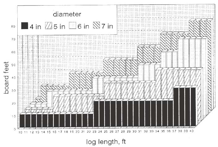
Based on these assumptions and ignoring taper, theoretical saw patterns were mapped for one inch log diameter classes. The total width of the theoretical boards in the sawing diagram, divided by 12, yields the number of board feet per lineal foot of log length for that diameter class. Scribner BF volumes are tabulated by multiplying the BF per lineal foot factor by log lengths (Anon. 1982a, b). The most prevalent form, Scribner Decimal C, occurs when the volumes are rounded to the nearest 10 BF. A portion of a Scribner table is given in Appendix 3. Some tables of this form are published without the zeros.
Since the assumed sawing patterns change with diameter only when boards can increase in width or when new boards can be added, the BF per lineal foot factors do not change smoothly with diameter. When this is combined with the practice of rounding to the nearest 10 BF, the resulting Scribner volumes change as a step function with log diameter and length (Figure 2-1). The erratic behavior of this step function results in many inconsistencies. For example:
-
A 4 inch diameter log always has a volume of 10 BF for any length between 8 and 22 feet, after which it doubles to 20 BF and remains constant for lengths to 36 feet, and so forth. Overrun, the difference between board feet of lumber actually recovered by a mill and the board feet predicted by Scribner, varies widely. At the beginning of a new step, overrun is low; it then climbs as the mill tally increases while the Scribner prediction is constant, and then abruptly declines when Scribner jumps to a new step.
-
The corresponding changes for 5 inch diameter logs have no consistent relation to the changes observed for 4 inch logs. All 4 and 5 inch logs have the same volume (10 BF) at lengths less than 15 feet and again (20 BF) at 23 feet, but differ elsewhere by 10 or 20 BF.
-
If a 4" x 20' log is cut into two 10 foot segments, the segments have a combined volume of 20 BF, double that of the original.
These inconsistencies occur throughout the range of log sizes and can create many problems. Loggers seeking to maximize scale will buck short lengths, thus constraining later utilization options. In an effort to prevent excessive "volume manufacturing," log buyers often stipulate a minimum average log length in contracts.
1. West-side (long log, coast, Bureau) Scribner
West-side Scribner is generally applied west of the Cascades in Washington and Oregon with the following procedure:
Diameteris measured inside bark at the small end. Two measurements are taken at right angles, with the short axis measured first and fractions of an inch are dropped. The resulting values are averaged and any fraction is dropped. This final result is the scaling diameter.
Length and trim: Logs are scaled in multiples of one foot length except when a "special service" request is made for two foot multiples. Gross length is taken from the short side of the log. No minimum trim is required. A maximum trim of 12 inches is allowed on lengths through 40 feet; an additional 2 inch trim is allowed for every 10 feet, or fraction thereof, exceeding 40 feet. When logs are scaled in two foot multiples under special service request, trim is required as given in the special service specifications.
Segment scaling: Logs 40 feet or less in gross length are scaled as a single piece (cylinder); taper is ignored. Logs 41 to 80 feet are scaled as two segments of as nearly equal gross length as possible; when two segments are not equal in length, the longer is the top (smaller diameter). Logs 81 to 120 feet in length are similarly scaled, except they are divided into three segments. Table 2-5 shows standard segment lengths and taper values (Anon. 1982b). In this table, taper is assumed to be 1 inch per 10 feet. The U.S. Forest Service differs from the table in that it uses actual taper to determine segment diameters (USFS 1977).
In assessing scaling defects to obtain net log scale, diameter or length is reduced depending on the type of defect.
2. East-side (short log, 20 foot maximum, inland, Forest Service) Scribner
East-side Scribner is applied in all other areas of the western United States, and log measurements and segment procedures are the same as described above (p. 17) for the Interagency Cubic Foot rule. Scribner volumes for each segment are found for the segment small end diameter and length; these volumes are summed to yield the total log volume.
In assessing scaling defects to obtain net scale, pie cut or squared defect procedures are used depending on the type of defect.
3. Comparing West-side and East-side Scribner
Figure 2-2 illustrates the differences in Scribner scale for a single log. It has 130 BF according to West-side practices and 210 BF according to East-side practices, a 62% difference. A bucker could "manufacture" a West-side scale increase by sawing the log into shorter segments. For example, if it were sawn in half, it would gain 40 BF (31%) with West-side scaling practices. However, if East-side scale were applied to the segments, there would be a loss of 20 BF. The nature of these effects is not consistent and must be evaluated on a log by log basis. The differences between East- and Westside Scribner have the following effects:
-
For 20 foot or shorter logs, the main difference in gross scale is the effect of dropping the fractional inch from the diameter measurement versus rounding the diameter. On a percentage basis, this effect is small for large diameter logs but ranges from 0 to 100% in small diameter logs.
-
For 21 to 40 foot logs, the differences due to diameter recording are compounded by the East-side procedure for using log taper and dividing logs into two scaling segments while the West-side system ignores taper and does not segment scale.
-
For logs longer than 40 feet, the pattern of differences changes again. West-side Scribner begins a two-segment scaling procedure with a fixed taper rate (except for USFS scaling, which uses actual taper) while East-side Scribner shifts from two to three scaling segments.
Table 2-5. Long log segment scaling for West-side Scribner.
Figure 2-2. Comparison of West-side and East-side
Scribner log scaling.
Example log: Small end dib = 10.7"
Large end dib = 16.3"
Length = 36' + trim
Midlength dib = 13.4"
West-side scale:
Single length 10" x 36' 130 BF

Bucked in half Piece #1 = 13" x 18' 110 BF
Piece #2 = 10" x 18' 60 BF
Total 170 BF
A 40 BF "manufactured" scale increase

East-side scale:
Single length Taper = 16" – 11" = 5"
Scale 2 segments 2" taper to butt log, 3" to top
Segment #1 = 14" x 18' 130 BF
Segment #2 = 11" x 18' 80 BF
Total 210 BF

Bucked in half Piece #1 = 13" x 18' 110 BF
Piece #2 = 11" x 18' 80 BF
Total 190 BF
A 20 BF "manufactured" scale loss

The differences and changes shown in this example would not necessarily be the same for logs of other dimensions. Each log presents a unique case as to how its actual geometry is handled by the procedures for treating diameters, segmenting, and taper.
Table 2-6 shows the 15 sample logs when scaled with the two forms of Scribner. Table 2-6 also presents conversion ratios between Scribner forms and the Interagency Cubic Foot rule (Table 2-3) and Japanese rules (Table 2-4). These ratios further illustrate the differences between the two Scribner forms and the variation in conversions in general. This particular log sample has a higher conversion between Scribner and Japanese rules than the 4.0 m3/MBF used in customs declarations and 5.6 m3/MBF to convert to JAS (p. 20).
4. Formulas to approximate Scribner
Knouf's rule:
BF = (d2 – 3d) L/20.
Girard and Bruce rule:
BF = 1.58d2 – 4d – 8 for 16
foot logs.
BF = 0.79d2 – 2d – 4 for 32 foot
logs.
Bruce and Schumacher rule (prorates the Girard and Bruce 16 foot formula to any length):
BF = (0.79 d2– 2d – 4) L/16
= 0.494 d2 L – 0.124 d L – 0.269
L.
Other Diagram Board Foot Log Rules. Spaulding (Columbia River) is similar to Scribner except that it has an 11/32 allowance for shrinkage and sawkerf. It is the statute rule in California. Humboldt is basically the Spaulding rule with a 30% reduction for defects. It has been widely used for redwood.
Log Rule Conversion Factors
Although a seemingly simple task, conversion between two log rules is highly variable. Tables 2-4 and 2-6 illustrate the high variability in log rule conversion ratios. This variability is due to:
-
Differences in how measurements are taken and recorded. Even when the same rule is being used, these differences may lead to a bias that would not otherwise exist. This is especially important internationally where countries may use the same formula but collect log data differently.
-
Differences in how volumes are recorded. Ignoring or assuming an incorrect rounding practice can cause bias.
-
Differences in formulas or rules used. Smalian's formula and the two-end conic rule do not yield the same cubic volume for a log even when all measurements are taken the same way.
-
The fact that log volumes change directly with length and with the square of diameter. Use of simple arithmetic averages can lead to bias. Tables 2-4 and 2-6 illustrate the difference in the conversion ratio based on using total volumes of all logs in the sample as opposed to averaging the volume ratios of the single logs.
Table 2-6. Scribner scaling of the 15 sample logs.
|
Ratio of
|
||||||||||
| Diameter |
Board feet/
|
Japanese rules to West-side
|
||||||||
| Small | Large | Length |
Scribner, BF
|
East/West | Interagency Cubic Foot |
Scribner (m3/MBF)
|
||||
|
|
||||||||||
|
(in)
|
(in)
|
(ft)
|
West
|
East
|
ratio
|
West
|
East
|
JAS
|
Hiragoku
|
South Sea
|
|
|
||||||||||
|
13.8 |
20.4 |
27.0 |
160 |
250 |
1.56 |
3.79 |
5.92 |
6.6 |
6.3 |
7.4 |
|
17.0 |
27.5 |
41.0 |
540 |
700 |
1.30 |
4.65 |
6.02 |
4.9 |
4.2 |
5.7 |
|
12.3 |
19.4 |
44.9 |
270 |
370 |
1.37 |
4.43 |
6.07 |
6.3 |
4.8 |
6.3 |
|
14.5 |
22.1 |
44.3 |
380 |
540 |
1.42 |
4.56 |
6.47 |
5.8 |
4.6 |
5.9 |
|
7.2 |
13.0 |
20.9 |
30 |
40 |
1.33 |
2.46 |
3.28 |
7.5 |
6.7 |
10.1 |
|
6.0 |
10.6 |
28.8 |
30 |
50 |
1.67 |
2.46 |
4.10 |
7.3 |
6.5 |
9.0 |
|
17.7 |
27.3 |
27.1 |
310 |
500 |
1.61 |
3.96 |
6.39 |
5.6 |
5.1 |
6.5 |
|
6.3 |
12.8 |
23.5 |
30 |
50 |
1.67 |
2.33 |
3.88 |
7.1 |
6.0 |
10.6 |
|
10.4 |
16.1 |
26.9 |
90 |
120 |
1.33 |
3.60 |
4.80 |
7.1 |
6.2 |
7.8 |
|
17.4 |
23.2 |
35.3 |
400 |
510 |
1.28 |
5.16 |
6.58 |
5.9 |
5.1 |
5.4 |
|
5.5 |
9.0 |
39.0 |
40 |
60 |
1.50 |
3.13 |
4.69 |
9.0 |
5.0 |
6.7 |
|
7.0 |
15.0 |
40.9 |
70 |
110 |
1.57 |
2.48 |
3.90 |
7.1 |
5.1 |
10.1 |
|
15.0 |
17.2 |
34.7 |
300 |
320 |
1.07 |
6.28 |
6.69 |
5.8 |
5.0 |
4.4 |
|
12.6 |
18.3 |
34.9 |
170 |
280 |
1.65 |
3.62 |
5.96 |
7.6 |
6.4 |
7.4 |
|
6.4 |
8.3 |
14.9 |
20 |
20 |
1.00 |
4.88 |
4.88 |
5.7 |
5.7 |
5.6 |
|
Total |
|
2,840 |
3,920
|
|||||||
|
Ratio of total volumes |
1.38 |
4.30 |
5.93 |
5.98 |
5.1 |
6.2
|
||||
|
Standard deviation |
0.21 |
0.91 |
0.72 |
1.02 |
0.82 |
1.21
|
||||
|
Coefficient of variation (%) |
15.0 |
21.2 |
12.1 |
17.1 |
16.2 |
19.6
|
||||
|
Sample precision (%) |
8.2 |
11.7 |
6.7 |
9.4 |
8.9 |
10.8
|
||||
|
Sample size for 2% precision |
216 |
432 |
140 |
279 |
251 |
369
|
||||
|
Average of individual log ratios |
1.42 |
3.85 |
5.31 |
6.62 |
5.51 |
7.26
|
||||
|
|
Conversions for Formula Log Rules: Algebraic Approach
When log rules are expressed as formulas, one approach is to form the ratio of the formulas, perform algebraic simplifications, and use the resulting expression. For example, the ratio of B.C. and Doyle BF log rules is
0.76 [(d – 1.5) / (d – 4)]2 .
To convert 5 million BF Doyle to the B.C. scale, assume that the average log diameter is 10 inches. The formula yields a B.C./Doyle ratio of 1.53, hence 5 million BF Doyle converts to 7.65 million BF in the B.C. rule. Suppose instead that data were available showing that the 5 million BF was distributed as follows:
|
Diameter (in)
|
Volume (%)
|
B.C./Doyle ratio
|
|
6-8
|
20
|
2.56
|
|
9-11
|
30
|
1.53
|
|
12-14
|
50
|
1.01
|
The weighted average conversion factor is
2.56 (0.20) + 1.53 (0.30) + 1.01 (0.50) = 1.48.
The 5 million Doyle now converts to 7.40 million BF in the B.C. rule. The additional information regarding the distribution of volume by diameter class resulted in a more refined estimate, which happens to be lower in this case.
This procedure of taking the ratio of log rule formulas and mathematically simplifying is valid only when both rules take and record log measurements in the same way and record resulting volumes with the same precision. Lacking these conditions, or as an alternative to the algebra, one can simply calculate volumes of individual logs under the alternative systems and develop a plot of the ratios. This approach could also be used when forming a ratio between a diagram rule and a cubic formula or between diagram rules, and so forth. When this is done, the plot is likely to be a disappointingly noisy scattergram, because of the previously discussed sources of variation.
Conversion Using Log Rule Tables
This approach can be used for any pair of rules and will be illustrated using the Scribner, Doyle, and International rules.
Suppose a shipment of logs has been scaled in West-side Scribner and the volume is 25 MMBF and the average log is 16 feet long and 14 inches in diameter. To convert to Doyle, use the log rule tables (Appendix 3) to find that the average log has 110 BF Scribner and 100 BF Doyle. Multiply the 25 MMBF Scribner by the Doyle-to-Scribner ratio for the average log (i.e., 100/110) to get 22.7 MMBF Doyle.
To convert the original Scribner to International, multiply 25 MMBF Scribner by the International-to-Scribner ratio for the average log (i.e., 135/110) to get 30.7 MMBF International.
The primary difficulty with this approach is discovering the dimensions of the average log. The procedure can be refined if the distribution of log sizes is known.
Sample Scaling for a Conversion Factor
It is difficult to develop a reliable conversion factor for a given batch or shipment of logs based on studying formulas and tables. The problems become worse when working with net scale, because additional variability is introduced by the process of making volume reductions due to defects. To develop a conversion factor with a stated reliability, statistical sampling methods must be used. Since a conversion factor is the ratio of two measures, statistical methods for ratio estimates are appropriate. Unfortunately, the simple basic formulas for mean and standard deviation are often incorrectly used, leading to biased results. This section illustrates ratio estimation procedures and simple random sampling to develop a conversion factor with a stated degree of reliability or precision. For further information or use of other sampling methods, a statistician should be consulted.
Let n = number of logs in a sample
Xi = volume of i-th log scaled with rule X
Yi = volume of i-th log scaled with rule Y
i = l, ..., n.
Assume that rule X volume is the numerator and rule Y volume is the denominator of the desired conversion factor (C). Then
C = ![]() /
/![]()
The variance of this ratio estimate can only be approximated, and the following formula is recommended (Cochran 1963; Mood et al. 1974):
VAR ![]() ~
~ 
A computational form for the standard deviation (SD) can be derived as
where 
The coefficient of variation (CV) percent is
CV = 100 * SD/C.
The coefficient of variation is a percent measure of log-to-log variability in the conversion factor. It may be known from previous samples or estimated from a preliminary sample from the logs of interest. The precision (error) of the sample conversion factor in percent is
P = CV ![]() .
.
This measures, in percent terms, how close the conversion factor, based on the sample, is to the true conversion factor one would know only by sampling every log in the population.
The value t is the Student's t statistic for the sample size n and a given probability level. If you wish to say that you are 95% certain that the sample-based conversion factor has P percent precision and sampled 30 logs, then t = 1.96.
The formula for precision can be rearranged to determine the size of sample needed to obtain a conversion factor that has a stated precision. This precision is often called reliability or allowable error.
n = (CV * t / P)2 (infinite population)
n = N (t2CV2) / (NP +
t2CV2)
(finite population, N = population size).
The required sample size will increase as the coefficient of variation increases; a larger sample will be needed to yield a factor with given reliability if there is less uniformity among the logs or between the rules in question. The required sample size will also increase as tighter allowable error and probability statements are imposed by the parties. The high variation observed in many log shipments, combined with tight statements desired by the parties, leads to large sample sizes. As a result, parties are often observed performing 100% scaling in both systems.
This section has presented methods based on simple random
sampling to the problem of developing a conversion factor between
any two log rules that has a stated measure of reliability. The
advantage of this approach lies in letting each log population
generate its own conversion, rather than assuming some arbitrary
or historical value that has not been verified and which may involve
large error. This is important since the resource base is changing
in both size and quality, and past experience may be irrelevant.
The main disadvantage of sample scaling is the need to
access the logs and measure the sample. There is a trade-off between
the cost of sampling and using a conversion factor that has not
been derived from or verified for the population at hand. It may
be possible to apply a different sampling system that may be more
efficient.
Example 4
Table 2-7 illustrates calculations for estimating a conversion factor between West-side Scribner and the Interagency Cubic Foot rule in which the 15 logs in the tables of this chapter are assumed to be a random sample from the population of interest.
|
Assuming the parties involved agree that they wish to be 95% certain that the conversion ratio is within 2% of the true conversion for the population, and assuming a large population, the infinite population formula yields a sample size of 432 logs. |
After pooling measurements of the 417 new logs with the original 15, suppose the conversion is 4.90 BF/ft3. The parties can say that they are 95% certain that the sample-based conversion of 4.90 is within 2% of the true conversion for the population. In other words, they are 95% sure that the true conversion for the population is between 4.8 and 5.0 BF/ft3.
Institutionalized Log Conversion Factors
In many cases, organizations and agencies develop and apply standard conversion factors. These may bear little relation to actual conditions, often have an obscure history, may be changed without notice, and frequently are not published. It is not the intention of this section to present and critique an exhaustive list of these, but it should be pointed out that differences between estimates of the same commodity reported by different agencies often are due in part to use of different conversion factors. For example, the discussion above on Scribner conversions (p. 20) indicated that Japanese statistics on exports of U.S. softwood logs are based on either 4.0 or 5.0 cubic meters/MBF West-side Scribner, depending on the reporting source.
Conversions Between Cubic Systems. Table 2-8 summarizes a number of standard conversions among various cubic systems and Brererton. These should be considered as approximate as they are theoretically correct only if the same formulas are used and measurements are taken and recorded in the same way. Tables 2-4 and 2-6 illustrate the high degree of variability that can occur among cubic systems and provides the motivation for sampling when an accurate conversion is needed.
|
Table 2-7. Example of conversion factor calculations for West-side Scribner to the Interagency Cubic Foot rule using the 15 sample logs.
Sx = 927,200 – 2,8402/15 = 389,493.3 Sy = 44,640.15 – 660.72/15 = 14,233.45733 Sxy = 181,821 – (2,730)(631.7)/15 = 66,851.6 C = 2,840/660.7 = 4.30 BF West-side Scribner per Interagency ft3 SD = 15 CV = P = 21.20 Suppose it is desired to have precision (allowable error) of 2%. The number of logs needed is n = Therefore, sample an additional 417 logs. |
||||||||||||||||||||||||||||||||||||||||||||||||||||||||||||||||||||||||||||||||||||||||||||||||||||||||||||||||||||||||||||||||||||||||||||||||||||||||||
Table 2-8. Cubic conversion factors.
|
Cubic foot |
Cubic meter |
Brererton |
|||||
|
|
|
||||||
|
From |
To |
Solid |
Hoppus |
Cunit |
Solid |
Francon |
BF |
|
|
|||||||
|
1 ft3, solid |
1 |
1.273 |
0.01 |
0.02832 |
0.0361 |
12 |
|
|
1 ft3, Hoppus |
0.785 |
1 |
0.00785 |
0.02223 |
0.02832 |
9.42 |
|
|
1 cunit |
100 |
127.3 |
1 |
2.832 |
3.608 |
1,200 |
|
|
1m3, solid |
35.315 |
44.987 |
0.353 |
1 |
1.273 |
424 |
|
|
1m3, Francon |
27.722 |
35.315 |
0.277 |
0.785 |
1 |
333 |
|
|
1 MBF, Brererton |
83.333 |
106.157 |
0.8333 |
2.360 |
3.00 |
1,000 |
|
|
|
|||||||
Conversions Between Brererton and Scribner. The U.S. Department of Commerce export regulations use the following conversion between West-side Scribner and Brererton:
MBF Scribner = 0.55 MBF Brererton.
MBF Brererton = 1.82 MBF Scribner.
This is based on the assumption of 6.6 BF Scribner per cubic foot (i.e., 6.6 BF Scribner/ft3 divided by 12 BF Brererton/ft3 = 0.55).
Conversions Between Board Feet and Cubic Feet or Cubic Meters. To convert 1,000 BF to cubic meters, divide 1,000 by the assumed ratio of board feet to cubic feet. Divide this result by 35.315 cubic feet per cubic meter to estimate the equivalent volume in cubic meters.
Perform these calculations for a series of BF/CF ratios:
BF/CF Cubic feet/MBF Cubic meters/MBF
3 333.33 9.44
4 250.00 7.08
5 200.00 5.66
6 166.67 4.72
7 142.86 4.04
8 125.00 3.54
9 111.11 3.15
10 100.00 2.83
11 90.91 2.57
12 83.88 2.36
Many organizations perform calculations of this nature.
Once one of these three ratios is estimated or assumed, the
others are readily calculated. Occasionally, values from the
last line are incorrectly applied to logs. This is erroneous
since it assumes that the entire cubic volume of the log is
expressed in board feet, a phenomenon that applies only in the
Brererton and Haakondahl rules.
In performing these calculations, the particular log rules for board feet or cubic feet were not specified. This can lead to problems of interpretation. For example, the sample logs in Table 2-6 have an average of 4.30 BF West-side Scribner per Interagency cubic foot. Dividing into 1,000 yields 232.6 Interagency cubic feet per MBF West-side Scribner. One would be tempted to conclude that this translates into about 6.6 cubic meters per MBF. However, if the sample logs are Hiragoku scaled in Japan, the proper conversion from Interagency cubic feet to Hiragoku for this sample is 45.99, not 35.315 (Table 2-4). Therefore, there are about 5.1 Hiragoku cubic meters per MBF West-side Scribner, which is the same value as the ratio of volume totals shown in Table 2-6. Note that every combination of a board foot rule and a cubic rule will yield a different result and that the results are sensitive to log size and taper. The above procedure can be used properly as long as users are very careful in their interpretation of which rules are involved and do not assume that 35.315 ft3/m3 applies to all combinations of cubic log rules.
Conversions Between Board Foot Systems. Appendix 2 presents log scale conversion factors used in the USFS assessment of the timber situation in the United States.
Log Weights
Cubic Foot Weight Scaling. The specific gravity and moisture content of a given species of wood can be used to calculate log weights when the log volume is known. The converse procedure of converting weight to volume is known as weight scaling. Since specific gravity and moisture content vary within and between species, many firms weigh and volume-scale loads of logs to develop proprietary weight-to-volume conversion factors. These are often stratified by species, source location, and season of year to account for some of the variation. Mann and Lysons (1972) present tables for estimating weight based on log diameter and length using a relationship they call a density index. Due to the large number of tables in their report, they are not reproduced here.
Board Foot Weight Scaling. Weight and board foot log rule measures are not closely related unless
diameter is taken into account. Paxson and Spaulding (1944) present weight/MBF Scribner Decimal C according to species and log diameter. The variation is large; for example, the range for Douglas-fir was from 5,200 to 13,500 lb/MBF. Unfortunately, their data do not extend into the smaller diameters characteristic of today's young growth; and current, published sources of this information are not available.
Log Weight Calculation. In the absence of log weight
tables, Chapter 1 (p. 7) presents procedures that can be used
to develop estimates.